VLSI Testing Lecture 4a: Logic Simulation

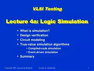
1. VLSI TestingLecture 4a: Logic Simulation • What is simulation? • Design verification • Circuit modeling • True-value simulation algorithms • Compiled-code simulation • Event-driven simulation • Summary Lecture 4a: Simulation

2. Simulation Defined • Definition: Simulation refers to modeling of a design, its function and performance. • A software simulator is a computer program; an emulator is a hardware simulator. • Simulation is used for design verification: • Validate assumptions • Verify logic • Verify performance (timing) • Types of simulation: • Logic or switch level • Timing • Circuit • Fault (Lecture 4b) Lecture 4a: Simulation

3. Simulation for Verification Specification Synthesis Response analysis Design (netlist) Design changes True-value simulation Computed responses Input stimuli Lecture 4a: Simulation

4. Modeling for Simulation • Modules, blocks or components described by • Input/output (I/O) function • Delays associated with I/O signals • Examples: binary adder, Boolean gates, FET, resistors and capacitors • Interconnects represent • ideal signal carriers, or • ideal electrical conductors • Netlist: a format (or language) that describes a design as an interconnection of modules. Netlist may use hierarchy. Lecture 4a: Simulation

5. c a e d f b HA D A Carry HA1 F E B HA2 Sum C Example: A Full-Adder HA; inputs: a, b; outputs: c, f; AND: A1, (a, b), (c); AND: A2, (d, e), (f); OR: O1, (a, b), (d); NOT: N1, (c), (e); Half-adder FA; inputs: A, B, C; outputs: Carry, Sum; HA: HA1, (A, B), (D, E); HA: HA2, (E, C), (F, Sum); OR: O2, (D, F), (Carry); Full-adder Lecture 4a: Simulation

6. Ca Logic Model of MOS Circuit VDD pMOS FETs a Da c Dc a b Db c Cc b Daand Dbare interconnect or propagation delays Dcis inertial delay of gate Cb nMOS FETs Ca , Cb and Cc are parasitic capacitances Lecture 4a: Simulation

7. Options for Inertial Delay(simulation of a NAND gate) Transient region a Inputs b c (CMOS) c (zero delay) c (unit delay) Logic simulation X rise=5, fall=5 c (multiple delay) Unknown (X) c (minmax delay) min =2, max =5 5 Time units 0 Lecture 4a: Simulation

8. Signal States • Two-states (0, 1) can be used for purely combinational logic with zero-delay. • Three-states (0, 1, X) are essential for timing hazards and for sequential logic initialization. • Four-states (0, 1, X, Z) are essential for MOS devices. See example below. • Analog signals are used for exact timing of digital logic and for analog circuits. Z (hold previous value) 0 0 Lecture 4a: Simulation

9. Modeling Levels Modeling level Function, behavior, RTL Logic Switch Timing Circuit Signal values 0, 1 0, 1, X and Z 0, 1 and X Analog voltage Analog voltage, current Application Architectural and functional verification Logic verification and test Logic verification Timing verification Digital timing and analog circuit verification Timing Clock boundary Zero-delay unit-delay, multiple- delay Zero-delay Fine-grain timing Continuous time Circuit description Programming language-like HDL Connectivity of Boolean gates, flip-flops and transistors Transistor size and connectivity, node capacitances Transistor technology data, connectivity, node capacitances Tech. Data, active/ passive component connectivity Lecture 4a: Simulation

10. True-Value Simulation Algorithms • Compiled-code simulation • Applicable to zero-delay combinational logic • Also used for cycle-accurate synchronous sequential circuits for logic verification • Efficient for highly active circuits, but inefficient for low-activity circuits • High-level (e.g., C language) models can be used • Event-driven simulation • Only gates or modules with input events are evaluated (event means a signal change) • Delays can be accurately simulated for timing verification • Efficient for low-activity circuits • Can be extended for fault simulation Lecture 4a: Simulation

11. Compiled-Code Algorithm • Step 1: Levelize combinational logic and encode in a compilable programming language • Step 2: Initialize internal state variables (flip-flops) • Step 3: For each input vector • Set primary input variables • Repeat (until steady-state or max. iterations) • Execute compiled code • Report or save computed variables Lecture 4a: Simulation

12. Event-Driven Algorithm(Example) Scheduled events c = 0 d = 1, e = 0 g = 0 f = 1 g = 1 Activity list d, e f, g g a =1 e =1 t = 0 1 2 3 4 5 6 7 8 2 c =1 0 g =1 2 2 d = 0 4 f =0 b =1 Time stack g 8 4 0 Time, t Lecture 4a: Simulation

13. Efficiency of Event-Driven Simulator • Simulates events (value changes) only • Speed up over compiled-code can be ten times or more; in large logic circuits about 0.1 to 10% gates become active for an input change Steady 0 0 → 1 event Large logic block without activity Steady 0 (no event) Lecture 4a: Simulation

14. Summary • Logic or true-value simulators are essential tools for design verification. • Verification vectors and expected responses are generated (often manually) from specifications. • A logic simulator can be implemented using either compiled-code or event-driven method. • Per vector complexity of a logic simulator is approximately linear in circuit size. • Modeling level determines the evaluation procedures used in the simulator. Lecture 4a: Simulation