Download
1 / 45
450 likes | 649 Views
An O(log n) Dominating Set Protocol for Wireless Ad-Hoc Networks under the Physical Interference Model. Andrea W. Richa Arizona State University Joint work with Christian Scheideler and Paolo Santi. Wireless Ad-hoc Networks . Mobile stations communicating over wireless medium Challenges:

E N D
An O(log n) Dominating Set Protocol for Wireless Ad-Hoc Networks under the Physical Interference Model Andrea W. Richa Arizona State University Joint work with Christian Scheideler and Paolo Santi
Wireless Ad-hoc Networks Mobile stations communicating over wireless medium Challenges: • design appropriate models • design and analyze algorithms under these models
Wireless Ad-hoc Networks • Wireless communication very difficult to model accurately • Signal propagation • Interference • Mobility • Physical Carrier Sensing • Algorithms are very difficult to analyze under a very accurate model Find balance between accuracy and provability.
UDG: What is the problem? Unit-Disk Graph (UDG) • Given a transmission radius R, nodesu, vare connected iff d(u,v) ≤ R Problems: • Transmission range could be of highly nonuniform shape • Does not consider interference u R v
u v' v w Packet Radio Network: What is the problem? • Can handle arbitrary transmission shapes • Nodes u, v can communicate directly iff they are connected. • Interference Model: • (interference range) = (transmission range) • Problem: linear slowdown if interference range is larger than transmission range
PRN: What is the problem? ≥ rt v s ≤ rt ≤ rt t ≤ ri n-2 nodes • While in the PRN model, s can send a message to t in 2 steps, no uniform protocol can successfully send a message in expected o(n) number of steps: linear slowdown
Bounded Interference Models Transmission and Interference Ranges: • Separate values. • Interference range constant times bigger than transmission range. • Problem? … u ri rt does not cause interference at u (even if all nodes outside transmit at the same time) may cause interference at u
Physical Interference Reality looks more like this: transmission range u interference
Bounded x Physical Interference: Bad News Bad news: • Blough, Canali, Resta, and Santi’08:combined interference from far-away nodes cannot be neglected • bounded interference model: neglected interference can be two orders of magnitude greater than noise floor • simulations: 210% loss in throughput when interference from far away nodes taken into account (We will see some good news later…)
Dominating Set Problem Classical dominating set problem: Given a graph G=(V,E) , find a subset U V of minimum size so that for every node v in V, either v is in U or v has a neighbor in U.
1 Dominating Set Problem Wireless setting: First formally analyzed for unit disk graph model.
Is dominating set problem still relevant in general setting? • Studies fundamental problem of selecting local leaders of constant density that cover entire network area. • Building block for many other problems in wireless networks. • constant density: at most a constant number of nodes in any constant size area. Our goal:Construct node set U of constant density via simple, local-control algorithm under the physical interference model so that all nodes vinV\U can receive messages from a node in U (i.e., U is coordinator set).
u Bounded x Physical Interference: Good news • Blough, Canali, Resta and Santi ’08:If nodes have constant density, then physical (SINR) interference model reduces to bounded interference model.
Overview of Talk • Our model • Signal propagation • Interference model • Physical carrier sensing • The dominating set problem • Our contribution • TWIN protocol • Algorithm • Analysis • Future Work
Signal Propagation Log-normal shadowing model: • d0: reference distance • >2: path loss coefficient • Signal loss at distance d in dB: -10 log(d/d0) + X for some Gaussian RV X
Signal Propagation Log-normal shadowing model without X : • P: signal strength at d0=1 • signal strength at distance d>1: P/d
Signal Propagation Our model: • Non-symmetric function c(v,w) [(1+)-1 d(v,w), (1+) d(v,w)] • accounts for nonuniform variations of communication environment • Received power (or signal strength) from v at w: Pw(v)=P/c(v,w)
Signal Propagation • random function c: approximates well (a truncated form of) the log-normal shadowing model
forward error correction: transition between being able to correctly receive a message (w.h.p.) and not being able to correctly receive a message (w.h.p.) is less than 1dB Transmission Range sharp boundary w v u
Physical Interference (SINR) • u receives msg from vif and only ifPu(v) N+w Pu(w)N: background noise • Received power from v at w: Pw(v)=P/c(v,w) > v u
Physical Carrier Sensing • Provided by Clear Channel Assessment (CCA) Circuit • Monitors the medium as a function of Received Signal Strength Indicator (RSSI) • Energy Detection (ED) bit set to 1 if RSSI exceeds a certain threshold • Has a register to set the threshold TSo v can check if N+w Pv(w) > T
Overview of Talk • Our model • Signal propagation • Interference model • Physical carrier sensing • Prior work and our Contribution • TWIN protocol • Algorithm • Analysis • Future Work
Prior Work Modelling: • Log-normal shadowing model and physical interference model common in physical layer community • Gupta and Kumar ’00, Grossglauser and Tse ‘01: capacity of wireless networks • Brar, Blough, Santi ’06 and Moscibroda, Wattenhofer, Zollinger ‘06: transmission scheduling • Goussevskaia, Moscibroda, Wattenhofer ’08: broadcasting Dominating sets: • Luby ’85, Alzoubi et al ’02, Dubhashi et al ’03, Kuhn et al ’03, Huang et al ’04,…: UDG • Kuhn et al ’04, Partasarathy and Gandhi ’04 : protocols for bounded interference model (runtime O(log2 n) ) • Kothapalli et al ‘05: protocol for more general bounded interference model with physical carrier sensing (runtime O(log4 n) )
Dominating Set Problem • V: set of n nodes of arbitrary distr. in IR2 • c: non-symmetric cost function • Find subset U of V of constant density so that for every v in V: • either v in U • or there is a w in U with Pv(w) > N. v can receive msg from w
Our Contribution • More general model for theoretical analysis (hopefully closer to reality) Theorem. TWIN protocol establishes a constant density dominating set in O(log n) time w.h.p. Main ideas: • Extensive use of physical carrier sensing • Leaders emerge in twins(if possible)
v Why Physical Carrier Sensing? • Using physical carrier sensing, we can extract information from the network without relying on successful message transmissions • quite often it is enough just to know if at least one node is sending a message, rather than receiving the message • linear speedup • It comes for “free”
Overview of Talk • Our model • Signal propagation • Interference model • Physical carrier sensing • The dominating set problem • Our contribution • TWIN protocol • Algorithm • Analysis • Future Work
TWIN Protocol • Nodes do not need any prior knowledge • All messages of constant size (signals) • All nodes transmit with same power P • Nodes may be • inactive: not in dominating set • twin: in dominating set; twins come up in pairs • active single: “isolated” nodes which cannot form a twin pair but are still needed for coverage • acc(v) : counter (acc(v)>0 iff vactive)
TWIN Protocol • Nodes operate in synchronized rounds that are continuously executed • Stage 1: announcing active twins • Stage 2: guessing the right density • Stage 3: forming new twins Diff frequency for each time slot: no sync round stage 1 stage 2 stage 3
TWIN Protocol For every node v: Initially, v is inactive and acc(v)=0. Access probability pv may have any value in (0, pmax], where pmax<<1. D: maximum density of twin nodes Stage 1: announcing active twins • Active twin: send ACTIVE signal with prob 1/D • Inactive or active single: if vreceives ACTIVE signal, it terminates and becomes inactive
TWIN Protocol 0<<1: constant inc/dec step for access probability Stage 2: guessing the right density • Inactive or active single: v chooses one of two time slots at random, say s (other slot s’). • Slot s:v sends PING signal with prob pv.If not, v senses channel with threshold T • Slot s’:v senses channel with threshold T • v does not senseanything: pv:=min{(1+)pv, pmax} • vsensesbusy channel: pv:=(1+)-1pv • If pv=pmax then acc(v):=acc(v)+4, elseacc(v):=max{acc(v)-1,0} (0: inactive) v is an active single
TWIN Protocol Stage 3: forming new twins • Inactive or active single: If vsent PING in slot s and received PING at slot s’in stage 2, then it sends ACK in slot s of this stage. If it receives an ACK signal in slot s’ of this stage, v becomes an active twin. v PING ACK w active twin active twin, since w must have received PINGfrom v only (otherwise no ACK from w) PING ACK
TWIN Protocol • (Stage 3.) If vjust became active twin, v sends NEW signal in last slot. If v is inactive or active single and senses a busy channel with threshold T, then v becomes inactive and terminates the protocol v NEW z inactive or active single inactive active twin sensing range of v
Overview of Talk • Our model • Signal propagation • Interference model • Physical carrier sensing • The dominating set problem • Our contribution • TWIN protocol • Algorithm • Analysis • Towards self-stabilization • Future Work
Analysis Overview • probabilities pv quickly converge to constant in every transmission area • low runtime: constant chance of twins emerging • constant twin density: twins must receive ACKs, and NEW signals deactivate local neighborhood • active singles: nodes not covered and not having node to pair up with eventually become active single; if density of active singles beyond certain constant, active twin will emerge
Getting Down to Constant Density • Sensing areaRs(v): • whenever a node in Rs(v) transmits, v will be able to sense transmission with threshold T • Rs(v) R(v), where R(v) is the transmission area of node v Lemma: After logarithmic many steps, w in RS(v) pw = O(1)for a constant fraction of the rounds. constant density
Bounding Far-away Interference bounded interference • A round is called good iff w in R(v) pw = O(1) and the interference caused by nodes not in R(v) is less than T-N • “far-away“ noise will not trigger busy channel • Lemma. For any constant ε>0, at least (1- ε) fraction of time steps are good for v w.h.p., if T sufficiently large.
Quick constant density coverage • Lemma. After a logarithmic number of steps, for a pmax<<1, every node v will • (coverage:)either be an active single or have an active twin within its transmission range, whp. Moreover, • (constant density:) have at most a constant number of active singles and twins within its transmission range whp
Conclusion • O(log n)-time protocol for dominating set under more realistic model • should be implementable in most simple devices • possible building block for many other applications on top of it Open questions: • self-stabilization • How does protocol perform in practice??? • More robust form (jamming-resistant)
Is the model sufficiently realistic? • Our interference model conservative: • signal cancellation • different signal strengths • bit recovery • fading and other nondeterministic characteristics of the wireless signal
Towards Self-Stabilization • Initial pv’s can be arbitrary • Initial acc(v)’s can be arbitrary Problems: • Termination of protocol not allowed.Instead, node should just “fall asleep” for O(log n) many rounds. • Initial density of active twins might be too high. Possible solution for 2.: add another time slot in which active twins check their cumulative signal strength (random decision to send or sense) Problem: time of stabilization cannot be bounded well, just eventual recovery
Self-Stabilization • wireless communication too complex: no model will be able to accurately take into account all that can happen Problem: What happens if things deviate from proposed model? Solution: Protocols need to be self-stabilizing, i.e., they need to go back to a valid configuration for the model