Download
1 / 42
420 likes | 554 Views
The physics of intergalactic gas. Serena Bertone serena@scipp.ucsc.edu March 9 th 2009. Overview. What is the IGM? Why do we care? IGM properties from simulations Low vs. high redshift IGM Observational techniques to detect the IGM: a bsorption lines emission lines F uture prospects

E N D
The physics ofintergalactic gas Serena Bertone serena@scipp.ucsc.edu March 9th 2009
Overview • What is the IGM? • Why do we care? • IGM properties from simulations • Low vs. high redshift IGM • Observational techniques to detect the IGM: • absorption lines • emission lines • Future prospects • References
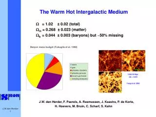
> 90% of the baryonic mass is in diffuse gas (Persic & Salucci 1992, Fukugita et al 1998, Cen & Ostriker 1999) Dark matter: 25% Metals: 0.03% Neutrinos: 0.3% Stars: 0.5% Free H & He: 4% Dark energy: 70%
Baryons in the Universe Prochaska & Tumlinson 2008
Why do we care about IGM? Fundamental ingredient in galaxy formation: • unbiased information on power spectrum of density fluctuations on largest scales • reservoir of fuel for star and galaxy formation • IGM metallicity constrains the cosmic star formation history • interplay IGM-feedback constrains galaxy formation models
How can we study the IGM? • with theory • with cosmological, hydrodynamicalsimulations of structure formation • with observations: • in the local universe • in the low redshift universe • in the high redshift universe
Basic recipe to simulate the IGM Ingredients: • initial conditions CMB • hydrodynamic physical model • numerical code Gadget, Enzo, Flash, Ramses… • big computer Shake well Evolution of gas density, temperature, metallicity, ionisation state etc… Mock observations
Springel 2003 z=6 z=2 z=0 IGM density evolution 100 Mpc cosmictime
Simulations have just about everything… Temperature Density Metallicity BUT: it doesn’t have to be correct! What you get is simply the result of the physics you put in
IGM temperature distribution at z=0 T<105 K 105 K <T<107 K T>107 K z=0 Cen & Ostriker 1999 • Warm-hot gas: WHIM • mildly overdense • collisionallyionised • shock heated by gravitational shocks • Hot gas: • dense • metal enriched • haloes of galaxies and clusters • Warm gas: • diffused • photo-ionised by UV background • traced by Lyα forest
Where are the baryons? What is the fraction of gas mass in given temperature/density ranges? How do these fractions evolve? • T>107 K hot cluster gas: small fraction @ all redshifts • 105 K<T<107 K WHIM: strongly increases with z • T<105 K diffuse Lyα forest gas: strong decrease • condensed: cold ISM + stars • Average IGM temperature increases with time Dave’ et al. 2001
Where are the metals? Simulations predict that: • most metals locked in stars at z=0 • most metals in star forming gas at z>2 • ~30% of metals in WHIM at all times • small fraction of metals in cool diffuse gas Wiersma et al 2009 How does this compare with observational results? halo gas diffuse IGM WHIM ICM
How can we detect the IGM? Temperature: wavelength of transition increases with temperature T=105 K @ z=0 O VI λ=1032Å T=106 K @ z=0 O VII λ=21.60Å T=107 K @ z=0 O VIII λ=18.97Å Example: oxygen IR optical UV X-rays wavelength T=105 K @ z=3 O VI λ=1032Å λ=4100Å Redshift: wavelength of transitions decreases with redshift
Absorption z<1: UV Tripp et al 2007 Lehner et al 2007 Danforth & Shull 2005 z>1.5: optical Kim et al 2001 Simcoe et al 2006 ✔ ? z<1 Nicastro et al 2005 Rasmussen et al 2007 Buote et al 2009 ✔ T<106 K Rest-frame UV lines Lyα, OVI, CIV… T>106 K Soft X-rays metal lines OVII, OVIII, FeXVII ✗ ✗ z<1: UV Furlanetto et al 2004 Bertone et al 2009a z>1.5: optical Weidinger et al 2004 Bertone et al 2009b z<1 Fang et al 2005 Bertone et al 2009a ✔✗ Emission
The Lyα Forest Absorption by warm photo-ionised gas along the LoS to a bright QSO Rest-frame UV lines: Lyα, C IV, O VI, N V, Si IV… 1-D information on: • spatial distribution of H I • spatial distribution of metal absorbers • column density of species gives information on: • temperature • density • metallicity • ionisation state John Webb UNSW Recovering this information is non-trivial!
Lyα forest evolution • Gas becomes hotter and progressively more ionised • Lyα forest becomes “thinner”: lines have lower column densities • overallspectrummovestoshorterwavelengths from optical to UV band Becker et al. 2001 “Neutral” IGM QSO 1422+23, zem=3.62 Wombleet al, 1996 wavelength (Angstroms) Tripp et al 2004 STIS, zem=0.3 wavelength (Angstroms)
The high-redshiftLyα forest • Rest-frame UV lines: • Lyman series lines: Lyα, Lyβ, Lyγ… • metal lines: C IV, O VI, N V, Si IV… • high resolution spectra from Keck and VLT needed for line properties • low resolution spectra (SDSS) good for power spectrum Kim et al 2001
UV absorption lines at z<1 • Current observations: FUSE, HST/STIS • Lyα, O VI and C IV narrow absorption lines prove prevalently cool and photoionised gas • Abundance of O VI at z<0.5 corresponds to Ωb(O VI) ~ 5-7% of baryons • Other UV lines: C IV, N V, Ne VIII, Si IV, Si III, C III… detectable with HST/COS Tripp et al 2007
Line density and opacity evolution Kim et al 2002 • number of absorption lines decreases with redshift • mean optical depth of lines decreases with redshift thinning of forest
Column density distributions • way to characterize the forest: number of lines vs. line column density • H I column density ≈ H I density, not hydrogen in general! • same analysis can be done for each species: C IV, O VI etc. Lyα forest z=3 z=0 LLS DLAs Column density distribution of ionised (Lyα forest) and neutral (DLAs, neutral H I and CO) gas. Prochaska & Tumlinson 2008
The Lyα forest power spectrum at z=2 • The flux power spectrum can be translated into the matter power spectrum of density fluctuations: τ ≈ ρα • the conversion is non-trivial: contamination from peculiar velocities, metal lines and non-linear structures (egDLAs) • flux power spectrum used with CMB and other data to estimate cosmological parameters Kim et al 2004
Baryonic mass density • fraction of baryons in the Lyα forest decreases with time • fraction of mass in stars increases with time • results comparable to predictions of simulations (see previous slides) • WHIM abundance not known observationally still missing! z=3 z=0 Estimates of baryonic mass densities, relative to Ωb, at z=3 and z=0. Prochaska & Tumlinson 2008
C IV mass density evolution • C IV abundance is NOT a prior for carbon • C IV abundance roughly constant with redshift up to z≈5 • C IV downturn at z≈6 indicates: • declining carbon abundance with z? • change in UV background? Ryan-Weber et al 2009
IGM metallicity Schaye et al 2003 Carbon abundance vs. overdensity Carbon abundance vs. redshift • Estimating the metallicity from ion abundances (eg C IV) requires non-trivial ionisation corrections • strong dependence on ionisingUV background • metallicity roughly depends on density of systems: lowest metallicity in lowest density regions and viceversa z=3 δ=0.5
The Lyα forest traces warm gas with T<105 K.What about the WHIM?
Broad Lyα absorptionlines (BLA) at z<1 Evidence of WHIM gas? • Lyα absorption fromcollisionallyionised gas with 105<T<106 K • Thermally broadened lines: bth> 40 km/s • upper limit on temperature STIS spectra (Richter et al 2006)
X-ray absorption lines z=0 absorbers Lines at z=0: what are they? • galactic halo? • local group gas? • nearby gas outside the local group? (Williams et al. 2005; Bregman 2007) Williams et al 2005 Chandra LETG spectrum of Mrk 421
The X-ray forest? Nicastro et al 2005 WHIM “detections” in X-rays are controversial 2-σ detection of two O VII absorption lines at z=0.011 and z=0.027 in the spectrum of Mkn 421 WHIM evidence or statistical fluke? Spectrum taken during QSO burst (Nicastro et al 2005). Detection not confirmed by XMM in deeper exposure (Rasmussen et al 2007). Statistical analysis not favorable (Kaastra et al 2006).
A real detection? • New strategy: look for absorption from known structures such as galaxy overdensities and filaments • Buote et al 2009: 3-σ detection of O VII absorption from Sculptor Wall at correct redshift • 3-σ still not extremely high significance… • More sensitive instruments needed! Buote et al 2009
X-ray emission @ z<1 • O VIII strongest line • lines from lower ionisation states and whose emissivity peaks at lower temperatures trace moderately dense IGM: C V, C VI, N VII, O VII,O VIII and Ne IX • lines from higher ionisation states trace denser, hotter gas: C VI, O VIII, Ne X, Mg XII, Si XIII, S XV and Fe XVII • Fe emission has different spatial distribution than other elements: later enrichment by SN Ia Bertone et al 2009a
UV emission@ z<1 • C IV strongest line: traces gas in proximity of galaxies • different spatial distribution: O VI and Ne VIII trace more diffuse gas than C IV • no emission from the hottest gas in groups Bertone et al 2009a
Rest-frame UV emission @ z>1.5 • At z>1.5 rest-frame UV lines are redshifted in to the optical band • A number of upcoming optical instrument might detect IGM emission lines at 1.5<z<5: • Cosmic Web Imager on Palomar (CWI, Rahman et al 2006) this year! • Keck Cosmic Web Imager (KCWI) • Antarctic Cosmic Web Imager (ACWI, Moore et al 2008) • MUSE on VLT (Bacon et al 2009) • IFUs with large fields of view & high spatial resolution • Great chance to observe the 3-D structure of the IGM for the first time!
Future prospects Currently, the IGM is only observed through rest-frame UV absorption lines at z<7 In the future it will be desirable to: • theory and simulations need to help understand observations several features still unexplained/not reproduced • understand shape,origin etc of UV background • detect the IGM in emission • detect the IGM in absorption in X-rays • detect the IGM in multiple bands multiphase gas? • extend surveys to higher redshifts (eg 21 cm line at z>7) • compare multi-wavelength data to obtain a deeper understanding of the physics of galaxy formation, as is currently done for galaxies
Wish-list of future instruments Detection of IGM in emission requires: • large field of view • high spatial resolution • high spectral resolution Telescopes to do the job: • X-ray missions: • Constellation-X & XEUS for absorption • EDGE, Xenia or better for emission • >10 years in the future • UV missions: • ISTOS or similar • > 5 years in the future • Optical instruments to study z>2: • CWI • KCWI or similar • 1 to 5 years in the future The missing baryons in the low redshift universe are the hardest to detect because of instrument requirements
CIV optical depth HI optical depth Feedback on the IGM Comparisons with IGM data help improve feedback models • C IV optical depth: indicator of C IV column density • Previous simulations (e.g. Springel & Hernquist 2003) were unable to predict the observed high column density of C IV at z>2 • Reason: metals are too hot in the simulations • Missing ingredients: • Metal cooling? Aguirre et al 2005; Wiersma et al 2009 • Wrong SN feedback model? Oppenheimer & Dave’ 2005+ BEFORE: no cooling LATER: metal cooling better agreement! Aguirre et al 2005
References • J.X. Prochaska & J. Tumlinson: Baryons: What, when and where? 2008, arXiv:0805.4635 • S. Bertone, J. Schaye, K. Dolag: Numerical simulations of the warm-hot intergalactic medium, 2008, SSR, 134, 259 • J. Bregman: The search for the missing baryons at low redshift, 2007, ARAA, 45, 221 • G. Stasinska: What can emission lines tell us?, 2007, Lectures XVIII Canary Islands Winter School • M. Rauch: The Lyα forest in the spectra of quasi-stellar objects, 1998, ARAA, 36, 267