K. Konstantinidis 1,2 , T. E. Sarris 1,2

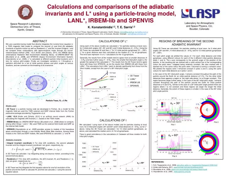
1. Calculations and comparisons of the adiabatic invariants and L* using a particle-tracing model, LANL*, IRBEM-lib and SPENVIS Laboratory for Atmospheric and Space Physics, CU, Boulder, Colorado Space Research Laboratory Democritus Univ. of Thrace, Xanthi, Greece K. Konstantinidis1,2, T. E. Sarris1,2 [1] Democritus University of Thrace, Space Research Laboratory, Xanthi, Greece, kkonst@ee.duth.gr, tsarris@ee.duth.gr [2] Laboratory for Atmospheric and Space Physics, Univ. of Colorado, Boulder, Colorado , sarris@lasp.colorado.edu ABSTRACT CALCULATIONS OF L* REGIONS OF BREAKING OF THE SECOND ADIABATIC INVARIANT We use a particle-tracing model that directly integrates the Lorentz-force equation in a TS05 magnetic field model to compute the second (J) and third (Φ) adiabatic invariants of particle motion as well as Roederer’s L* and the Invariant Integral I, and we compare these computations with approximations made through the neural-network-based method LANL* V2.0 [Koller and Zaharia, 2011], the IRBEM library (International Radiation Belt Environment Modeling library; ex-ONERA-DESP lib) [Bourdarie et al., 2008], and SPENVIS (Space Environment Information System) [Heynderickx et al., 2005]. L* is calculated at different particle initial locations and I also for various pitch-angles. Finally we investigate variations in I throughout a particle’s drift-shell for a set of initial particle phases and pitch angles at various locations, and we comment on the breaking of its invariance. Using each of the above models we calculated L* for particles starting at local noon, for 3 initial pitch angles (30o, 60o and 90o) and 5 initial distances (4 – 8 RE). Using the 3D Tracer we calculated Φ and then L* for 12 initial particle gyrophases (0o – 330o). L*for a given distance was then calculated as the median of L*for all gyrophases. The error bars represent 1σ of L*calculations for the 12 gyrophases. Generally, the results from all the models tend to agree more at smaller distances (4 – 6 RE) and less further away (7 – 8 RE). Also, the smaller theinitial pitch angle is, the greater the spread of the calculated L*. The results from the 3D Tracer tend to agree more with those from SPENVIS, as do the results from IRBEM LIB with those from LANL*. The calculations from LANL* seem to deviate significantly from those from the other models, except from the case of a 90o initial pitch angle. Using 3D Tracer we calculated I for particles starting at local noon, for 2 initial pitch angles (30o and 60o), 4 initial distances (5 – 8 RE) and for 12 initial particle gyrophases (0o – 330o). For each pitch angle we plotted the values of I for each initial distance and initial gyrophase, using different colours for each of the 4 different initial particle distances (plots 1 and 3). The x-axis corresponds to the azimuth angle of the position of the particle. In the resulting plot we marked with a solid vertical line of the corresponding colour the point were I stopped being relatively constant. We also marked with a dashed line of the same colour the point were I returned to having a constant value. We plotted the regions were I remained constant in plots 2 and 4, using the same colours for each initial distance as in plots 1 and 3. In the case of the 30o initial pitch angle, I remains constant throughout the path of the particle around the Earth for an initial particle distance of 5 RE. For the other initial distances there appears a region at the night side where I is no longer constant. This region becomes larger further away. In the case of the 60o initial pitch angle, I remains constant throughout the path of the particle around the Earth for initial particle distances of 4 and 5 RE. Similar to the case of a 30oinitial pitch angle particle there are regions where I is not constant and these regions are larger the longer the initial distance. Generally, the extent of these regions is smaller in the case of the 60o initial pitch angle particle. α0 = 30ο 8 RE 7 RE Particle Trace, Ri = 5 Re α0 = 30o 5 RE 6 RE 6 RE 7 RE • Models used: • 3D Tracer is a particle tracing code we developed in Fortran. As a model for the magnetic field we used the TS05 external and IGRF internal fields from the Fortran subroutine package provided by Tsyganenko et al. • LANL* V2.0 [Koller and Zaharia, 2011] is an artificial neural network (ANN) for calculating the magnetic drift invariant, L*, based on the TS05 model. • IRBEM library (ex ONERA-DESP library) [Bourdarie et al., 2008] allows to compute, among other things I and L*. We used TS05 as the external field model and IGRF as the internal field model. • SPENVIS [Heynderickx et al., 2005] provides access to models of the hazardous space environment through a user-friendly World Wide Web interface. Among these models is the TS05 and IGRF models. We used SPENVIS to calculate I, L* and Φ. α0 = 60ο α0 = 90ο 8 RE 5 RE CALCULATIONS OF I Plot 2 We calculated I using each of the above models and for particles starting at local noon, for 2 initial pitch angles (30o and 60o) and 5 initial distances (4 – 8 RE), as for L* above. Using the 3D Tracer we calculated I for 12 initial particle gyrophases, as above, and calculated the median and σ of Ifor all gyrophases. There is great coincidence in the calculations of I between all three models for both initial pitch angles. Plot 1 8 RE α0 = 60o 7 RE • Adiabatic invariants: • Integral invariant coordinate I: For slow drift conditions, the second adiabatic invariant and the integral invariant coordinate I are given, respectively, by: • and , where • In 3D Tracer we calculate I by integrating along one bounce motion, according to the second formula above. • Roederers L*: For slow drift conditions, the drift invariant, Φ, and Roederers L* (L-star) are given, respectively, by: • and • In 3D Tracer we first integrate the first equation above for one full revolution of the particle around the Earth to calculate Φ, and then we calculate L* using the second equation above. 6 RE 5 RE Plot 4 Plot 3 REFERENCES: 1. N.A. Tsyganenko et al., 2008, geo.phys.spbu.ru/~tsyganenko/Geopack-2008.html 2. Koller and Zaharia, 2011, www.lanlstar.lanl.gov/download.shtml 3. Bourdarie et al., 2008, irbem.svn.sourceforge.net/viewvc/irbem/trunk 4. Heynderickx et al., 2005 , www.spenvis.oma.be α0 = 30ο α0 = 60ο