Download

1 / 24
240 likes | 331 Views
Employing Grid Technology for Data Analysis Contact : www.business.duq.edu/faculty/davies. Computation Solutions. Traditional High-Performance Computer (HPC) Pro: Node-node communication Con: 20x to 200x cost of other solutions Traditional Cluster Computer

E N D
Employing Grid Technology for Data Analysis Contact: www.business.duq.edu/faculty/davies
Computation Solutions Traditional High-Performance Computer (HPC) Pro: Node-node communication Con: 20x to 200x cost of other solutions Traditional Cluster Computer Pro: Less expensive to maintain & upgrade Con: Requires significant infrastructure Internet Grid Computer Pro: Massive power on demand Con: Less adequate for massive data Enterprise Grid Computer Pro: Harness existing infrastructure Con: Limited power
Price per GF for HPC-Generated Computation Worldwide (excluding Departmental class) Installed base of HPC 400,000 GF* Annual cost of installed base $16.2 billion Average annual cost per GF $41,000 *1 gigaflops = 1 billion calculations per second ~ 5 GHz
Cluster Costs 20-Node Cluster Computer Purchase price per node $1,100 Effective life 3 years Weight (including racks) 1 ton Power consumption 8 kilowatts Required air conditioning 1 ton Required space 16 square feet Computational power 12 GF
Price per GF for Cluster-Generated Computation Total = $2,300 per GF per year $763 / year for nodes (amortized purchase price) $533 / year for labor $125 / year for installation and configuration (amortized) $33 / year for space $466 / year for electricity $275 / year for additional hardware (amortized) $69 / year for software (amortized) $69 / year for hardware service contracts Annual cost of a cluster > 125% of the (unamortized) purchase price of the nodes
Price Comparison Annual Cost per GF Traditional HPC $41,000 Traditional Cluster $2,300 Internet Grid $300* *Assumes ½ availability at $100 per year. What can a researcher do with cheap computation?
Exhaustive Regression (in the literature, “all subsets regression”) Goal: Examine all combinations of factors that have a significant effect on an outcome variable. Evaluate each combination on its ability to predict the outcome variable. Scope: With K factors, there are 2K possible factor combinations. There are statistical issues associated with performing data searches in this manner. But, in the absence of a theoretical model, the alternative is to do nothing.
Factor Combinations Example: Examine all combinations of three factors that might predict presence of natural gas. Rock Pyrolysis Organic Mass Spectrometry Outcome variable Potential Factors Presence of Natural Gas Vitrinite Reflectance
Factor Combinations Example: Examine all combinations of three factors that might predict presence of natural gas. Combination #1 Rock Pyrolysis Organic Mass Spectrometry Vitrinite Reflectance Combination #4 Organic Mass Spectrometry Vitrinite Reflectance Combination #5 Rock Pyrolysis Combination #2 Rock Pyrolysis Organic Mass Spectrometry Combination #6 Organic Mass Spectrometry Combination #3 Rock Pyrolysis Vitrinite Reflectance Combination #7 Vitrinite Reflectance
Factor Combinations As the number of possible factors grows, the number of models in the search space rises exponentially.
Factor Combinations Time requirement to exhaust all factor combinations with 40 factors when a single PC can compute 1,000 models per second 40 factors implies over 1 trillion possible models. Typically, researchers would use “stepwise procedures” to avoid having to compute all 1 trillion models.
Stepwise Procedures Model Quality Bad Poor Better Good Best Search Space Each square represents one combination of factors (a “model”). The 144 squares shown here correspond (approximately) to all the possible models that can be constructed using just 7 factors.
Stepwise Procedures Model Quality Bad Poor Better Good Best Starting here… * x …stepwise finds this model. Search Space Stepwise methods pick a single model as a starting point and follows an “improvement path” to a local optimum.
Stepwise Procedures Model Quality Bad Poor Better Good Best Search Space x x * x * * * x In this example, depending on where stepwise begins its search, stepwise could return any one of these four models.
Stepwise Procedures Stepwise methods would not reveal: Search Space • That there are four locally optimal models. • That there are five models that are as good as the local optima but are not themselves locally optimal. • That there are nine models that are ranked “Good” or “Best.” • Commonalities among the more preferred models. • Commonalities among the less preferred models.
Exhaustive Regression Exhaustive regression looks at all the models in the search (either within an OLS or LOGIT framework) and: 1. Returns results from all models, or 2. Returns only results from models that contain no insignificant parameter estimates, and/or 3. Returns only models that satisfy a specified minimum goodness of fit.
Exhaustive Regression • Models can be evaluated via: • Multiple correlation, • k-Fold cross-validation mean squared prediction error, or • Other methods List of factors that appear in each model. Each row corresponds to one of the 2K models.
Exhaustive Regression Proposed “other method”: Cross-model stability measure • Assuming: • The list of potential factors does not exclude any factors that determine the outcome variable, and • The pair-wise between-factor correlations are randomly distributed… …the expected values, across models, of parameter estimates will equal the values of the parameters.
Exhaustive Regression In preliminary Monte-Carlo experiments in which there are three “true” factors (among a set of up to 12 factors), the cross-model procedure correctly identifies: 1. All three of the “true” factors 85% of the time, and 2. Two of the three “true” factors 100% of the time. (moderate-low correlated data sets; average “true” R2 = 0.43)
Exhaustive Regression: Case Study Case Study: Amarillo Biosciences Problem: Amarillo Biosciences collected patient data from a phase II clinical study. Repeated statistical analyses of their experimental drug yielded no conclusive evidence for or against the drugs efficacy. With patient data comprising 36 factors, there were almost 69 billion possible ways to model the data.
Exhaustive Regression: Case Study Case Study: Amarillo Biosciences Solution: Looking at all 69 billion models, Exhaustive Regression revealed… • 250 models in which all factors were statistically significant, • 8 models that were superior (by stepwise criteria) to the single model found by stepwise methods, • 15 factors that were more stable (w.r.t. the cross-model criterion) than were the factors that stepwise methods selected, • 42 factors that did not appear in any of 250 significant models.
Employing Grid Technology for Data Analysis Contact: www.business.duq.edu/faculty/davies