Download
1 / 24
240 likes | 468 Views
Using Microsoft Excel. Under “Start”, go to “Programs” and select “Microsoft Excel”. Go the next slide to see the Excel Screen template. Row. Column. In using Excel, the first concept to understand is the “cell”. A Cell is the box created by the intersection of a row and a column.

E N D
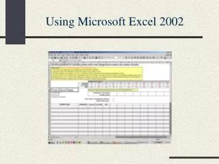
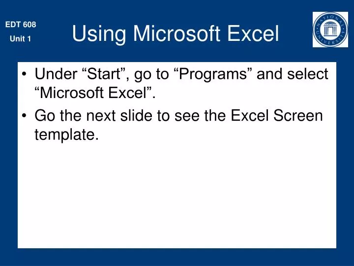
Using Microsoft Excel • Under “Start”, go to “Programs” and select “Microsoft Excel”. • Go the next slide to see the Excel Screen template.
Row Column • In using Excel, the first concept to understand is the “cell”. • A Cell is the box created by the intersection of a row and a column. • For example, where the column “A” and the row “1” intersect is cell “A1”.
To select a cell, place your cursor in the cell and click on it, The cell box will be bolded. (click for next slide)
Using an Excel Spreadsheet • Notice the information in the red and blue circles. • The red circle is an example of using the “Sigma” function to add. • The blue circle is an example of writing a formula to compute. Click to the next slide for illustrations of each
Sigma Symbol • Place your cursor in cell B9 and click. • Move your cursor on the “Sigma” symbol and click. • Upon the first click on the Sigma symbol, you will see the formula displayed in the cell as shown. • Click on the Sigma symbol a second time and the sum of all the numbers in the row will be automatically calculated and placed in cell B9. Go to the next slide to see the result. Cell B9
Next, we will calculate the sum of the same numbers by writing a formula for the numbers previously noted by the blue circle. Please go to the next slide.
Writing Formulas • The symbol for adding is a plus sign • The symbol for subtraction is a minus sign • The symbol for multiplying is an asterisk • The symbol for multiplying is a forward slash. • Note: When writing a formula, always start it with the “equals” sign or the software will not recognize your numbers as a formula. • Examples • =5*2 is a formula • 5*2 is not a formula • Please go to the next slide
Using cell locations to write a formula • It is often easier to use the cell locations of the number rather than the actual number in writing a formula. • The formula for calculating the quotient of 2 times 5 is therefore =D4*E4 • Once you have written the formula, then place your cursor in any empty cell and click. • The formula will be calculated and the answer placed in the cell where the formula was written. • Please go to the next slide to see the results.
Once the formula has been executed and the resulting figure placed in the cell, you can always check the formula by again placing your cursor over that figure and clicking. Please go to the next slide to see the result.
Formula Box • Determining the formula in a cell • Place your cursor in the cell and click. • The formula appears in the formula box at the top of the page
Shaded area with number of row which is 6 Lower line • Modifying the spreadsheet • You can make the width of the row wider by clicking on the lower line of the shaded area containing the number (e.g. 6) and dragging in out and releasing it or you can make it smaller by moving the line in and then releasing it. Go to next slide
Click on right line of box, hold, and drag out to desired width. Shaded Area Similarly, you can change the width of a column in the same manner You can also change the size of the font which will in-turn change the size of the cell. Go to the next slide for an illustration.
When you change the size of the font from 14 to 20, the size of the cell is expanded automatically to accommodate the new size.
Finally, please note that the menu bars are much the same as the ones you have used in MS Word and Power Point.
Using the MS Excel spreadsheet to do basic calculations • If you click the cursor in cell B11 and then click on • the sigma symbol, you will see the calculation • formula automatically written into the cell as noted in • the second grouping of numbers. • If you click the sigma symbol a second time, the • formula will automatically be computed and the • the result inserted into the cell. Please go to the next cell
Here is a practical use of an Excel spreadsheet in your classroom. • Some advantages are: • If you do a proposed budget but then find out that the price changes, simply delete the old price and insert the new one and the total will automatically be recalculated. • You can copy and paste and the formulas will remain in tact as in the case of the Second Semester budget that was copied from the First Semester Budget and pasted below it; the prices were changed but the total was recalculated automatically and the budget item name didn’t have to be retyped.
You can also use a Excel to compute the average of grades. • Note the formula written to compute the average of the five grades. • One the formula is written in cell G3 for Jimmy Johnson, you can click and hold your cursor on the lower right hand corner of the cell and drag it straight down to Tommy Fielding and the formula will be automatically inserted into each cell and the average automatically computed. • Please see the next slide.
The formula and average computation for these cells were automatically entered when the formula for cell G3 was dragged down through the cells.
The last application function of the Excel spreadsheet that we will review is that of “sorting”. • Notice that the students above are not in alphabetical order. • To sort them into alphabetical order, highlight all of the names. • On the menu bar at the top of the page click on “Data”.
Click on “Sort” Please go to next slide
When you click on “Sort” • A screen will appear like the one to the right. • There are two choices. • The “Expand the Selection” choice should automatically be selected for you, but if not, select it. • By selecting “Expand the Selection, the particular scores of each student is appropriately sorted to match the student. • Click on “Sort”
Another screen will appear and ask how you want the data to be sorted. Select Sort Column A Ascending (from A to Z). Click “OK”
Notice the names have been sorted alphabetically and the scores of each student moved appropriately.
End of MS Excel Tutorial • If you are not familiar with Excel, copy this presentation and use it as a guide/checklist to do some basic calculations and sorting. • Study of this presentation should provide you with sufficient information to complete it successfully.