Download
1 / 40
460 likes | 1.3k Views
Design of Engineering Experiments Part 7 – The 2 k-p Fractional Factorial Design. Text reference, Chapter 8 Motivation for fractional factorials is obvious; as the number of factors becomes large enough to be “interesting”, the size of the designs grows very quickly

E N D
Design of Engineering Experiments Part 7 – The 2k-p Fractional Factorial Design • Text reference, Chapter 8 • Motivation for fractional factorials is obvious; as the number of factors becomes large enough to be “interesting”, the size of the designs grows very quickly • Emphasis is on factorscreening; efficiently identify the factors with large effects • There may be many variables (often because we don’t know much about the system) • Almost always run as unreplicated factorials, but often with center points DOX 6E Montgomery
Why do Fractional Factorial Designs Work? • The sparsity of effects principle • There may be lots of factors, but few are important • System is dominated by main effects, low-order interactions • The projection property • Every fractional factorial contains full factorials in fewer factors • Sequential experimentation • Can add runs to a fractional factorial to resolve difficulties (or ambiguities) in interpretation DOX 6E Montgomery
The One-Half Fraction of the 2k • Section 8-2, page 283 • Notation: because the design has 2k/2 runs, it’s referred to as a 2k-1 • Consider a really simple case, the 23-1 • Note that I =ABC DOX 6E Montgomery
The One-Half Fraction of the 23 For the principal fraction, notice that the contrast for estimating the main effect A is exactly the same as the contrast used for estimating the BC interaction. This phenomena is called aliasing and it occurs in all fractional designs Aliases can be found directly from the columns in the table of + and - signs DOX 6E Montgomery
Aliasing in the One-Half Fraction of the 23 A = BC, B = AC, C = AB (or me = 2fi) Aliases can be found from the definingrelationI = ABC by multiplication: AI = A(ABC) = A2BC = BC BI =B(ABC) = AC CI = C(ABC) = AB Textbook notation for aliased effects: DOX 6E Montgomery
The Alternate Fraction of the 23-1 • I = -ABC is the defining relation • Implies slightly different aliases: A = -BC, B= -AC, and C = -AB • Both designs belong to the same family, defined by • Suppose that after running the principal fraction, the alternate fraction was also run • The two groups of runs can be combined to form a full factorial – an example of sequential experimentation DOX 6E Montgomery
Design Resolution • Resolution III Designs: • me = 2fi • example • Resolution IV Designs: • 2fi = 2fi • example • Resolution V Designs: • 2fi = 3fi • example DOX 6E Montgomery
Construction of a One-half Fraction The basic design; the design generator DOX 6E Montgomery
Projection of Fractional Factorials Every fractional factorial contains full factorials in fewer factors The “flashlight” analogy A one-half fraction will project into a full factorial in any k – 1 of the original factors DOX 6E Montgomery
Example 8-1 DOX 6E Montgomery
Example 8-1 Interpretation of results often relies on making some assumptions Ockham’srazor Confirmation experiments can be important Adding the alternatefraction – see page 294 DOX 6E Montgomery
The AC and AD interactions can be verified by inspection of the cube plot DOX 6E Montgomery
Confirmation experiment for this example: see pages 295-296 Use the model to predict the response at a test combination of interest in the design space – not one of the points in the current design. Run this test combination – then compare predicted and observed. For Example 8-1, consider the point +, +, -, +. The predicted response is Actual response is 104. DOX 6E Montgomery
Possible Strategies for Follow-Up Experimentation Following a Fractional Factorial Design DOX 6E Montgomery
The One-Quarter Fraction of the 2k DOX 6E Montgomery
The One-Quarter Fraction of the 26-2 Complete defining relation: I = ABCE = BCDF = ADEF DOX 6E Montgomery
The One-Quarter Fraction of the 26-2 • Uses of the alternate fractions • Projection of the design into subsets of the original six variables • Any subset of the original six variables that is not a word in the complete defining relation will result in a full factorial design • Consider ABCD (full factorial) • Consider ABCE (replicated half fraction) • Consider ABCF (full factorial) DOX 6E Montgomery
A One-Quarter Fraction of the 26-2:Example 8-4, Page 298 • Injection molding process with six factors • Design matrix, page 299 • Calculation of effects, normal probability plot of effects • Two factors (A, B)and the AB interaction are important • Residual analysis indicates there are some dispersion effects (see page 300) DOX 6E Montgomery
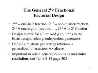
The General 2k-p Fractional Factorial Design • Section 8-4, page 303 • 2k-1 = one-half fraction, 2k-2 = one-quarter fraction, 2k-3 = one-eighth fraction, …, 2k-p = 1/ 2p fraction • Add p columns to the basic design; select p independent generators • Important to select generators so as to maximizeresolution, see Table 8-14 page 304 • Projection (page 306) – a design of resolution R contains full factorials in any R – 1 of the factors • Blocking (page 307) DOX 6E Montgomery
The General 2k-p Design: Resolution may not be Sufficient • Minimum abberation designs DOX 6E Montgomery
Resolution III Designs: Section 8-5, page 312 • Designs with main effects aliased with two-factor interactions • Used for screening (5 – 7 variables in 8 runs, 9 - 15 variables in 16 runs, for example) • A saturated design has k = N – 1 variables • See Table 8-19, page 313 for a DOX 6E Montgomery
Resolution III Designs DOX 6E Montgomery
Resolution III Designs • Sequential assembly of fractions to separate aliased effects (page 315) • Switching the signs in one column provides estimates of that factor and all of its two-factor interactions • Switching the signs in all columns dealiases all main effects from their two-factor interaction alias chains – called a full fold-over • Defining relation for a fold-over (page 318) • Be careful – these rules only work for Resolution III designs • There are other rules for Resolution IV designs, and other methods for adding runs to fractions to dealias effects of interest • Example 8-7, eye focus time, page 315 DOX 6E Montgomery
Remember that the full fold-over technique illustrated in this example (running a “mirror image” design with all signs reversed) only works in a Resolution II design. Defining relation for a fold-over design – see page 318. Blocking can be an important consideration in a fold-over design – see page 318. DOX 6E Montgomery
Plackett-Burman Designs • These are a different class of resolution III design • The number of runs, N, need only be a multiple of four • N = 4, 8, 12, 16, 20, 24, 28, 32, 36, 40, … • The designs where N = 12, 20, 24, etc. are called nongeometric PB designs • See text, page 319 for comments on construction of Plackett-Burman designs DOX 6E Montgomery
Plackett-Burman Designs See the analysis of this data, page 321 Many effects are large. DOX 6E Montgomery
Plackett-Burman Designs Projection of the 12-run design into 3 and 4 factors All PB designs have projectivity 3 (contrast with other resolution III fractions) DOX 6E Montgomery
Plackett-Burman Designs • The alias structure is complex in the PB designs • For example, with N = 12 and k = 11, every main effect is aliased with every 2FI not involving itself • Every 2FI alias chain has 45 terms • Partial aliasing can greatly complicate interpretation • Interactions can be particularly disruptive • Use very, very carefully (maybe never) DOX 6E Montgomery
Resolution IV and V Designs (Page 322) A resolution IV design must have at least 2k runs. “optimal” designs may occasionally prove useful. DOX 6E Montgomery
Sequential Experimentation with Resolution IV Designs – Page 325 We can’t use the full fold-over procedure given previously for Resolution III designs – it will result in replicating the runs in the original design. Switching the signs in a single column allows all of the two-factor interactions involving that column to be separated. DOX 6E Montgomery
The spin coater experiment – page 326 DOX 6E Montgomery
[AB] = AB + CE We need to dealias these interactions The fold-over design switches the signs in column A DOX 6E Montgomery
The aliases from the complete design following the fold-over (32 runs) are as follows: Finding the aliases is somewhat beyond the scope of this course (Chapter 10 provided details) but it can be determined using Design-Expert. DOX 6E Montgomery
A full fold-over of a Resolution IV design is usually not necessary, and it’s potentially very inefficient. In the spin coater example, there were seven degrees of freedom available to estimate two-factor interaction alias chains. After adding the fold-over (16 more runs), there are only 12 degrees of freedom available for estimating two-factor interactions (16 new runs yields only five more degrees of freedom). A partial fold-over (semifold) may be a better choice of follow-up design. To construct a partial fold-over: DOX 6E Montgomery
Not an orthogonal design Correlated parameter estimates Larger standard errors of regression model coefficients or effects DOX 6E Montgomery
There are still 12 degrees of freedom available to estimate two-factor interactions DOX 6E Montgomery
Resolution V Designs – Page 331 We used a Resolution V design (a 25-2) in Example 8-2 Generally, these are large designs (at least 32 runs) for six or more factors Irregular designs can be found using optimal design construction methods Examples for k = 6 and 8 factors are illustrated in the book DOX 6E Montgomery