Download
1 / 35
350 likes | 1.31k Views
Data acquisition. . Data acquisition. Using Cogent to a generate marker pulse.. drawpict(2); outportb(888,2); tport=time; waituntil(tport 100); outportb(888,0); logstring( [

E N D
1. Preprocessing for EEG & MEG Tom Schofield & Ed Roberts
2. In this experiment, the subject is being presented with letters on a screen. Mainly Xs, but sometimes the occasional O will appear.
The EEG is continually recorded from the subject by the digitization computer. It is amplified during the recording process, and often filtered in order to remove very high and very low frequency activity.
Stimulus PC presents stimulus to subject. As it presents each stimulus, the stimulus PC sends a pulse to the recording computer through a parallel port connection, telling it that a particular stimulus has been presented at a particular timeIn this experiment, the subject is being presented with letters on a screen. Mainly Xs, but sometimes the occasional O will appear.
The EEG is continually recorded from the subject by the digitization computer. It is amplified during the recording process, and often filtered in order to remove very high and very low frequency activity.
Stimulus PC presents stimulus to subject. As it presents each stimulus, the stimulus PC sends a pulse to the recording computer through a parallel port connection, telling it that a particular stimulus has been presented at a particular time
3. Data acquisition Using Cogent to a generate marker pulse..
drawpict(2);
outportb(888,2);
tport=time;
waituntil(tport+100);
outportb(888,0);
logstring( [�displayed �O� at time ' num2str(time) ]); This marker pulse is recorded in the data, marking when each stimulus is presented, and what type of stimulus it is.
This is how you generate it with cogent. In this example the �drawpict� command in the script tells the stim PC to display picture �2� and the �outportb� command tells the recording computer to make a record in the data stream that picture �2� was displayed at this timeThis marker pulse is recorded in the data, marking when each stimulus is presented, and what type of stimulus it is.
This is how you generate it with cogent. In this example the �drawpict� command in the script tells the stim PC to display picture �2� and the �outportb� command tells the recording computer to make a record in the data stream that picture �2� was displayed at this time
4. Two crucial steps Activity caused by your stimulus (ERP) is �hidden� within continuous EEG stream
ERP is your �signal�, all else in EEG is �noise�
Event-related activity should not be random, we assume all else is
Epoching � cutting the data into chunks referenced to stimulus presentation
Averaging � calculating the mean value for each time-point across all epochs The EEG data is recorded continuously, if the activity generated in response to the �X� or the �O� is the �signal� that you want, then the EEG activity not related to presentation of these stimuli can be characterised as �noise�.
If we assume that this noise is randomly occurring, then by epoching our data � by splitting it up into single trials referenced to stimulus presentation and then averaging these epochs together, point-by-point, the noise should cancel out and the activity related to the stimulus should become visible The EEG data is recorded continuously, if the activity generated in response to the �X� or the �O� is the �signal� that you want, then the EEG activity not related to presentation of these stimuli can be characterised as �noise�.
If we assume that this noise is randomly occurring, then by epoching our data � by splitting it up into single trials referenced to stimulus presentation and then averaging these epochs together, point-by-point, the noise should cancel out and the activity related to the stimulus should become visible
5. Extracting ERP from EEG ERPs emerge from EEG as you average trials together Here�s an example of this approach. On the left there are single EEG epochs. 4 epochs where an X was presented, 2 where an O was presented. All the epochs are different, there�s not much of a pattern apparent. But if you look at what happens when we start to average them together we start to see things more clearly. On the right on the top is the result if you average 80 x trials together. On the right underneath is what happens if you average 20 O trials together. As you can see, stimulus specific waveforms seem to be emerging. The most striking difference between the two conditions in this case is in the magnitude of the P3 component. If this difference is large enough, and there are enough trials, you�d probably be able to find a statistically significant difference between the two types of trial. Here�s an example of this approach. On the left there are single EEG epochs. 4 epochs where an X was presented, 2 where an O was presented. All the epochs are different, there�s not much of a pattern apparent. But if you look at what happens when we start to average them together we start to see things more clearly. On the right on the top is the result if you average 80 x trials together. On the right underneath is what happens if you average 20 O trials together. As you can see, stimulus specific waveforms seem to be emerging. The most striking difference between the two conditions in this case is in the magnitude of the P3 component. If this difference is large enough, and there are enough trials, you�d probably be able to find a statistically significant difference between the two types of trial.
6. Overview
Preprocessing steps
Preprocessing with SPM
What to be careful about
What you need to know about filtering
7. First step. Raw data from EEG or MEG needs to be put into format suitable for SPM to read.
So in SPM, you select �Convert�.
Tell SPM to expect data generated by a particular type of system by selecting from a list that pops up. Systems used at the FIL are; BDF for EEG and CTF for MEG.
Select the raw data file.
Select the data template file which contains information about the spatial locations of the electrode position
You then tell SPM if you want to read the whole file in. This is because if you�re recording MEG data at quite high sample rates, MATLAB can only handle data from about 15 minutes worth of recording. If you try to convert the whole thing and it crashes, you can try reading in half of it at a time.
Creates a .mat and a .dat file. The .mat file contains information about the structure of the data. The .dat file contains the data itself.First step. Raw data from EEG or MEG needs to be put into format suitable for SPM to read.
So in SPM, you select �Convert�.
Tell SPM to expect data generated by a particular type of system by selecting from a list that pops up. Systems used at the FIL are; BDF for EEG and CTF for MEG.
Select the raw data file.
Select the data template file which contains information about the spatial locations of the electrode position
You then tell SPM if you want to read the whole file in. This is because if you�re recording MEG data at quite high sample rates, MATLAB can only handle data from about 15 minutes worth of recording. If you try to convert the whole thing and it crashes, you can try reading in half of it at a time.
Creates a .mat and a .dat file. The .mat file contains information about the structure of the data. The .dat file contains the data itself.
8. Epoching Epoching splits the data into single trials, each referenced to stimulus presentation
For each stimulus onset, the epoched trial starts at some user-specified pre-stimulus time and ends at some post-stimulus time, e.g. from 100 ms before to 600ms after stimulus presentation.
You have to be careful with specifying your epoch timing. The epoched data is usually baseline corrected, the mean value in pre-stimulus time is subtracted from the whole trial. Essentially, you want your pre-stimulus interval to only contain noise. If there�s any activity related to the previous stimulus still around, it will be removed from the current epoch and you�ll distort your data.
Epoching splits the data into single trials, each referenced to stimulus presentation
For each stimulus onset, the epoched trial starts at some user-specified pre-stimulus time and ends at some post-stimulus time, e.g. from 100 ms before to 600ms after stimulus presentation.
You have to be careful with specifying your epoch timing. The epoched data is usually baseline corrected, the mean value in pre-stimulus time is subtracted from the whole trial. Essentially, you want your pre-stimulus interval to only contain noise. If there�s any activity related to the previous stimulus still around, it will be removed from the current epoch and you�ll distort your data.
9. Epoching - SPM So in SPM you select �Epoch�
You tell it how long post stimulus you want your epoch, and you tell it how long you want your baseline period to be.
Tell it which marker codes to look out for in order to segregate the trial types.
If you don�t have marker codes in your data, you can read in a list of times at which your events happened
You end up with a new .mat file which has an �e� attached to the front of it.So in SPM you select �Epoch�
You tell it how long post stimulus you want your epoch, and you tell it how long you want your baseline period to be.
Tell it which marker codes to look out for in order to segregate the trial types.
If you don�t have marker codes in your data, you can read in a list of times at which your events happened
You end up with a new .mat file which has an �e� attached to the front of it.
10. Downsampling Nyquist Theory � minimum digital sampling frequency must be > twice the maximum frequency in analogue signal
Select �Downsample� from the �Other� menu Recording MEG/EEG involves converting the analogue signal from the brain into a series of digital representations. The EEG/MEG does not really consist of continuous data. Data are sampled at a rate specified before recording e.g. 400 samples per second. A typical EEG consists of a sequence of thousands of discrete values, one after the other.
You have to sample at a high frequencies to get a good quality digital conversions of analogue signals. The minimum sampling frequency needs to be greater than twice the maximum frequency of any analogue signal likely to be present in the EEG. This is called the Nyquist frequency. In this figure, the top picture shows well sampled data. Each dot is a digital recording of the value of the wave at each time point. Underneath, there�s an example of under-sampling. The sampling is too sparse to capture the nature of the analogue wave. With a sampling frequency that�s too low, a signal of lower frequency is generated -- this phenomenon is known as aliasing
This means you are probably going to end up sampling your data at a higher resolution than you actually need to capture you components of interest. Once your data is safely digitised, you can downsample it so that it takes up less room and is quicker to work with.Recording MEG/EEG involves converting the analogue signal from the brain into a series of digital representations. The EEG/MEG does not really consist of continuous data. Data are sampled at a rate specified before recording e.g. 400 samples per second. A typical EEG consists of a sequence of thousands of discrete values, one after the other.
You have to sample at a high frequencies to get a good quality digital conversions of analogue signals. The minimum sampling frequency needs to be greater than twice the maximum frequency of any analogue signal likely to be present in the EEG. This is called the Nyquist frequency. In this figure, the top picture shows well sampled data. Each dot is a digital recording of the value of the wave at each time point. Underneath, there�s an example of under-sampling. The sampling is too sparse to capture the nature of the analogue wave. With a sampling frequency that�s too low, a signal of lower frequency is generated -- this phenomenon is known as aliasing
This means you are probably going to end up sampling your data at a higher resolution than you actually need to capture you components of interest. Once your data is safely digitised, you can downsample it so that it takes up less room and is quicker to work with.
11. Downsample SPM uses the matlab function RESAMPLE to downsample your data. You select �Downsample� from the �Other� menu and tell it the new sampling rate you want. And it creates a new .mat file with a �d� appended to it.
SPM uses the matlab function RESAMPLE to downsample your data. You select �Downsample� from the �Other� menu and tell it the new sampling rate you want. And it creates a new .mat file with a �d� appended to it.
12. Artefact rejection Blinks
Eye-movements
Muscle activity
EKG
Skin potentials
Alpha waves
Some epochs will be contaminated with activity that does not come from brain processes.
Major artefacts are � eyeblinks, eve-movements, muscle activity, changes in skin impedance, alpha waves. These will all contaminate your data to some extent.
Within each eye there is an electrical gradient, positive at the front. Movement of the eyelids across the eye modulates the conduction of this electrical potential of the eyes to the surrounding regions.
Moving the eye itself actually changes the electrical gradients observable at the scalp, making them more positive in the direction the eye has moved towards. Also moves stimulus across retina, this generates unwanted visual ERPs.
Muscle activity is characterised by bursts of high frequency activity in the EEG.
EKG reflects activity of the heart. This can intermittently appear in your data
Skin potentials are only really a problem for EEG. They reflect changes in skin impedence, this could happen if the subject starts to sweat more as the experiment progresses. They look like slow drifts.. Sometimes if they drift far enough, they cause saturation of the amplifier - a flat �blocking� line.
Alpha waves are actually generated by the brain. They�re slow repetitive waves of about 10 hz which are unlikely to be of any interest to you if you�re looking at cognitive processes.Some epochs will be contaminated with activity that does not come from brain processes.
Major artefacts are � eyeblinks, eve-movements, muscle activity, changes in skin impedance, alpha waves. These will all contaminate your data to some extent.
Within each eye there is an electrical gradient, positive at the front. Movement of the eyelids across the eye modulates the conduction of this electrical potential of the eyes to the surrounding regions.
Moving the eye itself actually changes the electrical gradients observable at the scalp, making them more positive in the direction the eye has moved towards. Also moves stimulus across retina, this generates unwanted visual ERPs.
Muscle activity is characterised by bursts of high frequency activity in the EEG.
EKG reflects activity of the heart. This can intermittently appear in your data
Skin potentials are only really a problem for EEG. They reflect changes in skin impedence, this could happen if the subject starts to sweat more as the experiment progresses. They look like slow drifts.. Sometimes if they drift far enough, they cause saturation of the amplifier - a flat �blocking� line.
Alpha waves are actually generated by the brain. They�re slow repetitive waves of about 10 hz which are unlikely to be of any interest to you if you�re looking at cognitive processes.
13. Artefact rejection Blinks
Eye-movements
Muscle activity
EKG
Skin potentials
Alpha waves
So are these artefacts going to be a big problem if they appear in our data?
Short answer is that we don�t really have to worry about muscle activity. Low-pass filter will deal with muscle artefact.
Heart artefact is in a similar frequency range to ERP components, so can�t be dealt with by filtering. Luckily, usually don�t really have to worry about it as it shouldn�t appear systematically - will come and go � probably just increase overall noise levels.
Same holds for alpha waves, unless individual is particularly sleepy.
Skin potentials only appear with EEG. Again, don�t really need to worry about them as they are usually rare, slow and random. Will just add a bit of noise.
This is an important point � assuming you have a high number of trials, and your artefact is not systematically stimulus-linked, then a simple averaging procedure is surprisingly good at eliminating artefact.
Biggest problems usually are eye-blinks and eye movements. In a visual paradigm, for example, the chances are that these will be stimulus-linked. How do we deal with them?
One way to do this is by rejecting epochs which you think are contaminated by artefact. The problem here lies in recognising when things like eye-blinks have occurred. Luckily most artefactual activity is different in pattern from brain related activity, usually of a larger amplitude
This means the simple method of thresholding can be used to reject epochs in which the EEG reading shows an amplitude of above a certain amount. Alternatively, you can use eye-tracking equipment to record eye events as they occur during the experiment, and then mark these epochs as contaminated.So are these artefacts going to be a big problem if they appear in our data?
Short answer is that we don�t really have to worry about muscle activity. Low-pass filter will deal with muscle artefact.
Heart artefact is in a similar frequency range to ERP components, so can�t be dealt with by filtering. Luckily, usually don�t really have to worry about it as it shouldn�t appear systematically - will come and go � probably just increase overall noise levels.
Same holds for alpha waves, unless individual is particularly sleepy.
Skin potentials only appear with EEG. Again, don�t really need to worry about them as they are usually rare, slow and random. Will just add a bit of noise.
This is an important point � assuming you have a high number of trials, and your artefact is not systematically stimulus-linked, then a simple averaging procedure is surprisingly good at eliminating artefact.
Biggest problems usually are eye-blinks and eye movements. In a visual paradigm, for example, the chances are that these will be stimulus-linked. How do we deal with them?
One way to do this is by rejecting epochs which you think are contaminated by artefact. The problem here lies in recognising when things like eye-blinks have occurred. Luckily most artefactual activity is different in pattern from brain related activity, usually of a larger amplitude
This means the simple method of thresholding can be used to reject epochs in which the EEG reading shows an amplitude of above a certain amount. Alternatively, you can use eye-tracking equipment to record eye events as they occur during the experiment, and then mark these epochs as contaminated.
14. Artefact rejection - SPM There are two ways to perform artefact rejection with SPM. You can use thresholding to tell it to reject every trial which contains an absolute value exceeding a certain amount. Or you can give it a list of trials which you know to be contaminated by artefact.
You select �artefact�, click yes to give it a list of contaminated trials, or click no just to threshold all trials. Then click �yes� to �threshold channels?� and then type in the threshold you want to use. To decide on the threshold, you could try looking at your epoched data and picking a value that seems sensible. This marks as bad all epochs that contain super-threshold activity and generates a new .mat file with an �a� at the front of it.
Unfortunately thresholding isn�t really a very sensitive way of detecting artefact. If it turns out not to be good enough for you � might have to write your own matlab script to run on your data outside SPM. You might tell it to look for peak-to-peak differences within an epoch of above a certain value, for example. Then you could read this list into SPM.
Or if you�re really worried about alpha waves contaminating your data, for example, you could ask matlab to look at each epoch in turn, perform a Fourier transform on it to give you a measure of the frequency profile of the epoch, and tell SPM to reject the entire epoch if the activity at 10hz is above a certain amount.There are two ways to perform artefact rejection with SPM. You can use thresholding to tell it to reject every trial which contains an absolute value exceeding a certain amount. Or you can give it a list of trials which you know to be contaminated by artefact.
You select �artefact�, click yes to give it a list of contaminated trials, or click no just to threshold all trials. Then click �yes� to �threshold channels?� and then type in the threshold you want to use. To decide on the threshold, you could try looking at your epoched data and picking a value that seems sensible. This marks as bad all epochs that contain super-threshold activity and generates a new .mat file with an �a� at the front of it.
Unfortunately thresholding isn�t really a very sensitive way of detecting artefact. If it turns out not to be good enough for you � might have to write your own matlab script to run on your data outside SPM. You might tell it to look for peak-to-peak differences within an epoch of above a certain value, for example. Then you could read this list into SPM.
Or if you�re really worried about alpha waves contaminating your data, for example, you could ask matlab to look at each epoch in turn, perform a Fourier transform on it to give you a measure of the frequency profile of the epoch, and tell SPM to reject the entire epoch if the activity at 10hz is above a certain amount.
15. Artefact correction Rejecting �artefact� epochs costs you data
Using a simple artefact detection method will lead to a high level of false-positive artefact detection
Rejecting only trials in which artefact occurs might bias your data
High levels of artefact associated with some populations
Alternative methods of �Artefact Correction� exist There are problems with the Artefact rejection approach. The main problem is that if you throw out all trials that might possibly contain artefact, you�ll end up with smaller datasets.
Additionally, the data that remains might well be from an unrepresentative sample of trials.
If you want to look at children, patients etc., you can expect a higher proportion of trials to be contaminated by artefact - and you�ll probably be collecting less data than you would with controls anyway. If you reject all artefact epochs in these cases, you�ll be lucky to have enough trials left to extract an ERP
In some cases, rather than throw out epochs which you think contain artefact, it might be a better idea to try to correct for it instead. There are problems with the Artefact rejection approach. The main problem is that if you throw out all trials that might possibly contain artefact, you�ll end up with smaller datasets.
Additionally, the data that remains might well be from an unrepresentative sample of trials.
If you want to look at children, patients etc., you can expect a higher proportion of trials to be contaminated by artefact - and you�ll probably be collecting less data than you would with controls anyway. If you reject all artefact epochs in these cases, you�ll be lucky to have enough trials left to extract an ERP
In some cases, rather than throw out epochs which you think contain artefact, it might be a better idea to try to correct for it instead.
16. Artefact correction - SPM SPM uses a robust average procedure to weight each value according to how far away it is from the median value for that timepoint Artefact correction methods also attempt to detect artefact, but instead of simply rejecting the whole epoch, they attempt to estimate the relative size of the artefact and correct it in the data This will leave more trials, therefore better S/N � the problem is that these corrections themselves can cause significant distortion if they are incorrectly estimated.
SPM uses a Robust Averaging Paradigm.
For each time point, the median value across all epochs is calculated. Then each data point at that time point is weighted according to how far away from the median it is.
Those within a certain range are weighted �1�, those further away are weighted lower, down to zero. The acceptable range varies according to how tightly distributed the points are about the median.
This procedure is run again, using the new weighted values to calculate the median, and the process iterates until the weighting values become constant.
In the picture here you can see the results of this process � Red points have been weighted �1�, as points get further away from the centre, they receive less weight.
These weighting values are written in the .mat file, to be used later when you average your data.
As it uses median values rather than mean values, it�s far more robust to outliers � which can have a disproportional effect on mean values. Artefact correction methods also attempt to detect artefact, but instead of simply rejecting the whole epoch, they attempt to estimate the relative size of the artefact and correct it in the data This will leave more trials, therefore better S/N � the problem is that these corrections themselves can cause significant distortion if they are incorrectly estimated.
SPM uses a Robust Averaging Paradigm.
For each time point, the median value across all epochs is calculated. Then each data point at that time point is weighted according to how far away from the median it is.
Those within a certain range are weighted �1�, those further away are weighted lower, down to zero. The acceptable range varies according to how tightly distributed the points are about the median.
This procedure is run again, using the new weighted values to calculate the median, and the process iterates until the weighting values become constant.
In the picture here you can see the results of this process � Red points have been weighted �1�, as points get further away from the centre, they receive less weight.
These weighting values are written in the .mat file, to be used later when you average your data.
As it uses median values rather than mean values, it�s far more robust to outliers � which can have a disproportional effect on mean values.
17. Artefact correction - SPM Normal average
Robust Weighted Average Here�s an average waveform derived from the data on the previous slide.
In red is what we get if we just average the values together without trying to identify outliers.
In blue is what we get if we use the weighting values for each data-point in our average
As you can see, several small artefactual peaks are eliminated by the procedureHere�s an average waveform derived from the data on the previous slide.
In red is what we get if we just average the values together without trying to identify outliers.
In blue is what we get if we use the weighting values for each data-point in our average
As you can see, several small artefactual peaks are eliminated by the procedure
18. Robust averaging - SPM To perform this, you select �Artefact�, click �No� when it asks if you want to read in your own artefact list
Then select robust average
Then select how strict you want it to be in its weighting. 3 is the default.
Then select the default smoothing option.
This will create a new .mat file with an �a� in front of it.
To perform this, you select �Artefact�, click �No� when it asks if you want to read in your own artefact list
Then select robust average
Then select how strict you want it to be in its weighting. 3 is the default.
Then select the default smoothing option.
This will create a new .mat file with an �a� in front of it.
19. Artefact Correction ICA
Linear trend detection
Electro-oculogram
�No-stim� trials to correct for overlapping waveforms
Other popular methods of artefact correction, these aren�t used by SPM so I won�t talk too much about them.
ICA for eyeblinks. This separates your data into what it thinks are the components driving your data. You then visually inspect each of these components and pick the one you think might represent eyeblinks. Your data is then rebuilt without this component.
Linear trend detection looks for slow drifts in your data and tries to remove these trends from your data
EOG technique records activity from electrodes placed under the eyes. This is assumed to give a good estimate of eye movements and blinks. A fraction of this value is then removed from the EEG to compensate for blinks.
It�s not strictly artefact, but If you�re looking at long latency waves, you might end up with substantial overlap between trials. If in your design you include trials where there are no stimuli, you can average together only these �no-stim� trials. Assuming these trials only contain activity from the preceding stimulus, you�ll then get an �overlap� wave that you can subtract from your other epochs.
20. Artefact avoidance Blinking
Avoid contact lenses
Build �blink breaks� into your paradigm
If subject is blinking too much � tell them
EMG
Ask subjects to relax, shift position, open mouth slightly
Alpha waves
Ask subject to get a decent night�s sleep beforehand
Have more runs of shorter length � talk to subject in between
Jitter ISI � alpha waves can become entrained to stimulus In practice, there are problems with both artefact rejection and artefact correction. It�s always best to try to minimize artefact in the first place.
Artefact from eye-movements becomes less important over areas further way from the eyes. With an auditory paradigm you might be justified in ignoring these artefacts.In practice, there are problems with both artefact rejection and artefact correction. It�s always best to try to minimize artefact in the first place.
Artefact from eye-movements becomes less important over areas further way from the eyes. With an auditory paradigm you might be justified in ignoring these artefacts.
21. Averaging R = Noise on single trial
N = Number of trials
Noise in avg of N trials
(1/vN) x R
More trials = less noise
Double S/N need 4 trials
Quadruple need 16 trials Once you�ve rejected or corrected the artefact in your data. You need to extract your ERP. Generally you�ll just perform a simple average of each point, or use the Robust averaging data to perform a weighted average.
We assume that the ERP �signal� is the same on all trials, and unaffected by the averaging process. And assume as we said earlier, that the noise is random.
On there left are 8 single trial EEG epochs. On the right is what happens as we average each trial together. We can see that as we add each trial to the average, the resulting waveform becomes more consistent.
S/N ratio actually increases as a function of the square root of the number of trials. So in practice, you need a huge number of trials to extract your signal. As a general rule, it�s always better to try to decrease sources of noise than it is to increase the number of trials.Once you�ve rejected or corrected the artefact in your data. You need to extract your ERP. Generally you�ll just perform a simple average of each point, or use the Robust averaging data to perform a weighted average.
We assume that the ERP �signal� is the same on all trials, and unaffected by the averaging process. And assume as we said earlier, that the noise is random.
On there left are 8 single trial EEG epochs. On the right is what happens as we average each trial together. We can see that as we add each trial to the average, the resulting waveform becomes more consistent.
S/N ratio actually increases as a function of the square root of the number of trials. So in practice, you need a huge number of trials to extract your signal. As a general rule, it�s always better to try to decrease sources of noise than it is to increase the number of trials.
22. Averaging Averaging is simple. You just click �average�, then select the file you want to perform the average on.
This will give you a new .mat file with a �m� at the front of itAveraging is simple. You just click �average�, then select the file you want to perform the average on.
This will give you a new .mat file with a �m� at the front of it
23. Averaging Assumes that only the EEG noise varies from trial to trial
But � amplitude will vary
But � latency will vary
Variable latency is usually a bigger problem than variable amplitude Extracting ERPs from EEGs in this manner relies on few assumptions that aren�t strictly true.
Perhaps the biggest false assumption is that the ERP remains constant for each trial. We also assume that the noise in the EEG signal varies randomly across the experiment. Neither of these assumptions are completely true.
Any two ERPs elicited by the same stimuli will vary from each other in both the peak amplitude of some components of the ERP, and in the latency of these components.
Variations in peak amplitude can be quite large � but in the end you�ll still get an ERP which accurately reflects the average amplitude of each component. Variations in latency have a more profound affect on the averaged waveform.Extracting ERPs from EEGs in this manner relies on few assumptions that aren�t strictly true.
Perhaps the biggest false assumption is that the ERP remains constant for each trial. We also assume that the noise in the EEG signal varies randomly across the experiment. Neither of these assumptions are completely true.
Any two ERPs elicited by the same stimuli will vary from each other in both the peak amplitude of some components of the ERP, and in the latency of these components.
Variations in peak amplitude can be quite large � but in the end you�ll still get an ERP which accurately reflects the average amplitude of each component. Variations in latency have a more profound affect on the averaged waveform.
24. Averaging: effects of variance Latency variation can be a significant problem Averaging ERPs that vary in latency can give you a severely unrepresentative wave form.
In general, the greater the variation in onset, the flatter and more spread out the resulting waveform
At the bottom left, the latency varies a little between trials, and we see that average wave is a lot squatter than any of the single trial waves.
With greater latency differences, as seen in the top left, the problem gets much worse.
Notice also that the onset and offset of the mean waveform are not the average onset and offset times of the underlying events.
The onset in the average wave is the earliest of all onsets from all epochs � the offset is the latest of all offsets.
The problem is the greatest when we�re dealing with multiphasic waveforms that differ in phase. In the worst case, the resulting average wave might be flat � all information is lost in the averaging procedure as negative phase in some trials occurs at the same peri-stimulus time as positive phase in others. Averaging ERPs that vary in latency can give you a severely unrepresentative wave form.
In general, the greater the variation in onset, the flatter and more spread out the resulting waveform
At the bottom left, the latency varies a little between trials, and we see that average wave is a lot squatter than any of the single trial waves.
With greater latency differences, as seen in the top left, the problem gets much worse.
Notice also that the onset and offset of the mean waveform are not the average onset and offset times of the underlying events.
The onset in the average wave is the earliest of all onsets from all epochs � the offset is the latest of all offsets.
The problem is the greatest when we�re dealing with multiphasic waveforms that differ in phase. In the worst case, the resulting average wave might be flat � all information is lost in the averaging procedure as negative phase in some trials occurs at the same peri-stimulus time as positive phase in others.
25. Latency variation solutions Don�t use a peak amplitude measure Simplest solution to this problem is to measure your waveforms differently.
Peak amplitude is poor measure to use in this sort of situation.
As an alternative, you could measure the area under the curves.
In both of the examples here, the area under the average curve is equal to the average area under the single trials curves.
This won�t give you a latency measurement, however.
If you draw a line which bisects the average curve, where there is 50% of the area on either side of the line, as shown in red on the figures, then this line will give you an average peak latency measurement for the single trial curves.
Neither of these approaches will work for the multiphasic wave we saw earlier, however, as in this case averaging throws away all the information present in the single trials. Simplest solution to this problem is to measure your waveforms differently.
Peak amplitude is poor measure to use in this sort of situation.
As an alternative, you could measure the area under the curves.
In both of the examples here, the area under the average curve is equal to the average area under the single trials curves.
This won�t give you a latency measurement, however.
If you draw a line which bisects the average curve, where there is 50% of the area on either side of the line, as shown in red on the figures, then this line will give you an average peak latency measurement for the single trial curves.
Neither of these approaches will work for the multiphasic wave we saw earlier, however, as in this case averaging throws away all the information present in the single trials.
26. Time Locked Spectral Averaging This is a method of extracting information from waves that vary in latency and phase.
Essentially, you use something called a wavelet to generate a map of the frequency activity that�s present in your data (what a wavelet is this will be covered next week). This shows information regardless of phase differences. In the plots show, the lighter parts represent frequencies that are particularly well represented at the timepoints on the x axis. On the left is a plot generated from looking at each trial individually, and then combining all the individual frequency maps. We can see that there�s a lot of 40hz activity at about 100ms, and also some at 300 ms.
The plot on the right is a time frequency map of the waveform generated after all epochs have been averaged together. The 40hz activity at 100ms is still there, but the activity at 300ms has disappeared, suggesting that this activity might reflect a multiphasic ERP component that appears at 300ms.
This is a method of extracting information from waves that vary in latency and phase.
Essentially, you use something called a wavelet to generate a map of the frequency activity that�s present in your data (what a wavelet is this will be covered next week). This shows information regardless of phase differences. In the plots show, the lighter parts represent frequencies that are particularly well represented at the timepoints on the x axis. On the left is a plot generated from looking at each trial individually, and then combining all the individual frequency maps. We can see that there�s a lot of 40hz activity at about 100ms, and also some at 300 ms.
The plot on the right is a time frequency map of the waveform generated after all epochs have been averaged together. The 40hz activity at 100ms is still there, but the activity at 300ms has disappeared, suggesting that this activity might reflect a multiphasic ERP component that appears at 300ms.
27. Other stuff you can do � all under �Other� in GUI Merge data sessions together
Calculate a �grand mean� across subjects
Rereference to a different electrode
FILTER
28. Filtering Why would you want to filter?
29. Potential Artefacts Before Averaging�
Remove non-neural voltages
Sweating, fidgeting
Patients, Children
Avoid saturating the amplifier
Filter at 0.01Hz
30. Potential Artefacts After Averaging�
Filter Specific frequency bands
Remove persistent artefacts
Smooth data
31. Types of Filter Low-pass � attenuate high frequencies
High-pass � attenuate low frequencies
Band-pass � attenuate both
Notch � attenuate a narrow band
32. Properties of Filters �Transfer function�
Effect on amplitude at each frequency
Effect on phase at each frequency
�Half Amp. Cutoff�
Frequency at which amp is reduced by 50%
Half amp. Cutoff, frequency at which amplitude is reduced by 50%, or in terms of power; power = 50%, when amp = 71%
Half amp. Cutoff, frequency at which amplitude is reduced by 50%, or in terms of power; power = 50%, when amp = 71%
33. High-pass Diminishes the larger peak due to filtering out the lower frequency components
Artefactual peaks introduced into the higher frequency components.Diminishes the larger peak due to filtering out the lower frequency components
Artefactual peaks introduced into the higher frequency components.
34. Low-pass Removes high frequency 30Hz + noise, gamma etcRemoves high frequency 30Hz + noise, gamma etc
35. Band-pass and Notch Band pass useful for selecting a band of frequencies, e.g. if you wanted to purely examine Beta or Theta oscillations.
Notch useful for removing a specific frequency e.g. 50Hz mains supply, or local interference source.Band pass useful for selecting a band of frequencies, e.g. if you wanted to purely examine Beta or Theta oscillations.
Notch useful for removing a specific frequency e.g. 50Hz mains supply, or local interference source.
36. Problems with Filters Original waveform, band pass of .01 � 80Hz
Low-pass filtered, half-amp cutofff = ~40Hz
Low-pass filtered, half-amp cutofff = ~20Hz
Low-pass filtered, half-amp cutofff = ~10Hz
Although the waveform at the bottom looks the smoothest, and perhaps nicest, it now contains very little information and doesn�t resemble the original very much.
Although the waveform at the bottom looks the smoothest, and perhaps nicest, it now contains very little information and doesn�t resemble the original very much.
37. Filtering Artefacts �Precision in the time domain is inversely related to precision in the frequency domain.� The sharp cut-off in the filter leads to distortion in the waveform, a change in the onset time, and extra oscillations which were not previously present.
A sharp cut-off would seem ideal, and specific, but in reality they cause more problems than they solve.The sharp cut-off in the filter leads to distortion in the waveform, a change in the onset time, and extra oscillations which were not previously present.
A sharp cut-off would seem ideal, and specific, but in reality they cause more problems than they solve.
38. Filtering in the Frequency Domain The 60 Hz component is attenuated and then reverse Fourier-transformed to return to the original waveform.The 60 Hz component is attenuated and then reverse Fourier-transformed to return to the original waveform.
39. Filtering in the Time Domain Filtering in the time domain is analogous to smoothing
At a given point an average is calculated in relation to two nearest neighbours or more Smooth by averaging with surrounding points.Smooth by averaging with surrounding points.
40. Filtering in the Time Domain Waveform progressively filtered by averaging the surrounding time points.
Here x = ((x-1)+x+(x+1))/3 The data in the bottom right plot is derived from the taking the smoothest curve away from the original, thus giving the high frequency noiseThe data in the bottom right plot is derived from the taking the smoothest curve away from the original, thus giving the high frequency noise
41. Recipe for Preprocessing
42. Recommendations Prevention is better than the cure
During amplification and digitization minimize filtering
Keep offline filtering minimal, use a low-pass
Avoid high-pass filtering
Clean data
During Amp and digitization process, minimise filtering, avoid notch filters
Minimise offline filtering, maybe just use a low-pass filter to clean data
Avoid high-pass filters, only occasionally useful, and nearly always problematic.Clean data
During Amp and digitization process, minimise filtering, avoid notch filters
Minimise offline filtering, maybe just use a low-pass filter to clean data
Avoid high-pass filters, only occasionally useful, and nearly always problematic.
43. Summary No substitute for good data
The recipe is only a guideline
Calibrate
Filter sparingly
Be prepared to get your hands dirty
Good data solves all your problems
Use this as a guideline, it varies with experiment, personal judgement to find an appropriate balance is necessary. Over processed data is not necessarily comparable with other peoples� data sets.
Calibration lets you know exactly what you are doing to your data, introducing phase shifts etc.
Less is more.
Batch scripts are available to do a lot of the processing, but writing a few lines of code in matlab will make sure you are in complete control. SPM is not 100% on this yet�Good data solves all your problems
Use this as a guideline, it varies with experiment, personal judgement to find an appropriate balance is necessary. Over processed data is not necessarily comparable with other peoples� data sets.
Calibration lets you know exactly what you are doing to your data, introducing phase shifts etc.
Less is more.
Batch scripts are available to do a lot of the processing, but writing a few lines of code in matlab will make sure you are in complete control. SPM is not 100% on this yet�
44. References An Introduction to the Event-related Potential Technique, S. J. Luck
SPM Manual