Download
1 / 77
790 likes | 1.31k Views
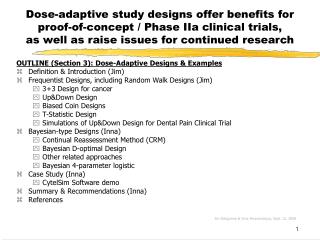
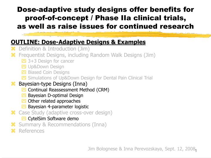
Dose-adaptive study designs offer benefits for proof-of-concept / Phase IIa clinical trials, as well as raise issues for continued research. OUTLINE: Dose-Adaptive Designs & Examples Definition & Introduction (Jim) Frequentist Designs, including Random Walk Designs (Jim) 3+3 Design for cancer

E N D
Dose-adaptive study designs offer benefits for proof-of-concept / Phase IIa clinical trials,as well as raise issues for continued research OUTLINE: Dose-Adaptive Designs & Examples • Definition & Introduction (Jim) • Frequentist Designs, including Random Walk Designs (Jim) • 3+3 Design for cancer • Up&Down Design • Biased Coin Designs • Simulations of Up&Down Design for Dental Pain Clinical Trial • Bayesian-type Designs (Inna) • Continual Reassessment Method (CRM) • Bayesian D-optimal Design • Other related approaches • Bayesian 4-parameter logistic • Case Study (adaptive cross-over design) • CytelSim Software demo • Summary & Recommendations (Inna) • References Jim Bolognese & Inna Perevozskaya, Sept. 12, 2008
Continual Reassessment Method (CRM) • Most known Bayesian method for Phase I trials • Underlying dose-response relationship is described by a 1-parameter function family • For a predefined set of doses to be studied and a binary response, estimates dose level (MTD) that yields a particular proportion (P) of responses • CRM uses Bayes theorem with accruing data to update the distribution of MTD based on previous responses • After each patient’s response, posterior distribution of model parameter is updated; predicted probabilities of a toxic response at each dose level are updated • The dose level for next patient is selected as the one with predicted probability closest to the target level of response • Procedure stops after N patients enrolled • Final estimate of MTD: dose with posterior probability closest to P after N patients • The method is designed to converge to MTD Innovative Clinical Drug Development Conference
Continual Reassessment Method (cont.) Choose initial estimate of response distribution & choose initial dose Update Dose Response Model & estimate Prob. (Resp.) @ each dose Obtain next Patient’s Observation Next Pt. Dose = Dose w/ Prob. (Resp.) Closest to Target level Stop. EDxx = Dose w/ Prob. (Resp.) Closest to Target level Max N Reached? no yes
Escalation With Overdose Control (EWOC) Bayesian Design • Assigns doses similarly to CRM, except for overdose control • predicted probability of next assignment exceeding MTD is controlled (Bayesian feasible design) • this distinction is particularly important in oncology • Assumes a model for the dose-response curve in terms of two parameters: • MTD • probability of response at dose D1 • EWOC updates posterior distribution of MTD based on this two-parameter model • Free software available here: • http://sisyphus.emory.edu/software_ewoc.php • Reference: • Z.Xu, M. Tighiouart, A. RogatkoEWOC 2.0: Interactive Software for Dose Escalation in Cancer Phase I Clinical Trials Drug Information Journal 2007 : 41(02) Babb, et al., 1998
Decision Theoretic Approaches • Similar to CRM • Incorporates elements of Bayesian Decision Theory • Designed to study a particular set of dose levels D1, . . ., Dk • Two-parameter model for dose response with prior distributions on the parameters • Loss function minimizes asymptotic variance of dose which yields a particular proportion of responses • Posterior distribution estimates of the 2 parameters used to derive next dose, i.e., that estimated to have desired response level Whitehead, et al., 1995
Bayesian D-Optimal Sequential Design • Based on formal theory of optimal design (Atkinson and Donev, 1992) • Similar to EWOC, a constraint is added to address the ethical dilemma of avoiding extremely high doses • Uses a two parameter logistic model for dose response curve • Slope & location • Binary endpoint • Minimum response rate fixed at 0%, maximum at 100% • Sequential procedure assigns dose at each stage which minimizes variance of posterior distribution of model parameters Haines, et al., 2003
Simulated Bayesian D-Optimal Design for ED50 (http://haggis.umbc.edu/cgi-bin/dinteractive/inna1.html) • Efficacy: Percent of patients with “Response” assumed underlying distribution Dose: 1 2 3 4 5 6 7 %Response: 30 40 55 65 75 75 75 • Prior estimates: ED25 between doses 1 and 2 ED50 between doses 2 and 3 • 6 patients in Stage 1 for seeding purposes • D-Optimal Design: 3 pts at dose 1, 2 at dose 3, 1 at dose 4 # responses: 1 1 1 • 24 subsequent patients (total 30 patients) entered sequentially at doses yielding minimum variance of model for ED50 estimate • Response / non-response assigned to approximate targeted %G/E distribution above
Simulated Bayesian D-Optimal Designfor ED50 – Results (http://haggis.umbc.edu/cgi-bin/dinteractive/inna1.html)
Simulated Bayesian D-Optimal Designfor ED50 – Summary • Results from a single implementation Dose: 1 2 3 4 5 6 7 assumed %Response: 30 40 55 65 75 75 75 #Responses: 4 - 2 1 8 - - #patients: 13 0 4 1 12 0 0 observed %Response: 31 - 50 100 67 - - • Bayesian estimated ED50 = dose 2.3 • However, few observations at other than 2 doses due to optimal design for particular dose-response model • Dose-Response curve between those two doses could be interpolated by the underlying fitted model • Should not extrapolate from model outside observed range • 2-parameter model (slope, location) forced through 0% and 100%
Bayesian Design for the 4-parameter Logistic model • Underlying model: Available doses: Yijis (continuous) response of the j-th subject on the i-thdose, di is the vector of parameters of the distribution f • Patients are randomized in cohorts • Within each cohort, fixed fraction (e.g. 25%) is allocated to placebo, • For the remaining patients within cohort, dose is picked adaptively out of • Doses are picked so that QWV (Quantile Weighted Variance) utility function is minimized Developed by S. Berry for CytelSim (~2006)
Bivariate Models: Penalized Adaptive D-optimal Designs • Addresses safety and efficacy simultaneously • Design is characterized by two dependent binary outcomes (efficacy and toxicity) • Similar to univariate model: involves dose-escalation and early stopping rules • Similar to Bayesian Sequential D-Optimal Design: • Model-based approach with formal optimality criteria: “maximize the expected increment of information at each dose” • Instead of Bayesian posterior update, Maximum Likelihood Estimates of current trial data used for next dose selection • “Penalized” design: Introduces various constraints that can be flexible to reflect ethical concerns, cost, sample size, etc. Dragalin, 2005
Bayesian-type DesignsPros (+) & Cons (-) + Minimize observations at doses of little interest (too small or large) + CRM assigns doses which migrate & cluster around EDxx - little info on dose-response away from targeted dose (e.g., ED50) + can compensate by targeting 2 or 3 response levels + Bayesian D-optimal design efficiently estimates model-based dose-response curve (& targeted EDxx) - yields most observations at 2 dose levels to optimally fit model - model restrictive - forced through 0% and 100% response levels - should not extrapolate response levels beyond observed doses
Bayesian-type DesignsPros (+) & Cons (-) - Subjective nature of assignment of prior (starting) distribution - could take many observations to overcome an incorrect prior - Models underlying current methods not general enough for efficacy endpoints - 4-parameter model needed to estimate min & max response levels - Co-factors not included; could confound estimates + execute designs within important co-factor levels - Computations complex; little software available - Difficult to explain to clients - Not yet proven substantially better than up-and-down or t-statistic s designs when aim is estimation of dose-response curve
Logistics for Conduct of a Dose-Adaptive Designed Trial • Response observable reasonably quickly • Increased statistical computations / simulations to justify dose-adaptive scheme in protocol • Need on-call person to assess previous response data and generate dose for next subject • For model-based dose-adaptive designs, need on-call unblinded statistician for associated analyses • OR, this could be automated via web-based interface (increases cost) • Rapid transfer of needed data • Need special packaging or unblinded pharmacist at site to package selected dose for each patient
Remarks (2) • Logistics of implementation more complicated than usual parallel group design • Frequent data calls / brief simple analyses • Close contact with sites re: dose assignments • Special packaging (IVRS??) • Drug Supply – needed sufficiently for many possibilities • Tolerability rule(s) can be added for downward dose-assignment if pre-specified AE criteria are encountered • This has been studied in context of Bayesian dose-adaptive designs, but not in context of up&down designs • Number of placebo patients maintained as designed for intended precision vs. that group; could be down-sized, though
Dose-Adaptive DesignSummary • Allocation of dose for next subject based on response(s) of previous subject(s) • Random Walk designs: only last subject’s response • T-statistic (frequentist) designs: all previous subjects’ responses • Bayesian-type designs: all previous subjects’ responses • High potential to limit subject allocation to doses of little interest (too high / too low) • Maximize information gathered from fixed N • Ethical advantage over fixed randomization • More attractive to patients / subjects • Inference conditional on doses assigned by design, but not overly important in early development • Requires more statistical up-front work (simulation) • No pre-specified allocation schedule; requires ongoing communication with site regarding allocation
Dose-Adaptive Design Summary • Bayesian-type designs preferable to estimate dose-response curve; can also estimate a dose-response quantile of interest (e.g., EDxx) or (part of?) region of increasing dose-response • Complex; heavy computations • Random Walk & T-statistic Designs focus on quantile(s) of interest • Easy to understand & program • Consider as starting point for implementing dose-adaptive design • Let other design features guide towards other adaptive techniques based on particular experimental situation • Ongoing incomplete simulations have yet to identify major advantage of Bayesian-type designs over RW & T, unless prior information is important to consider. • Study, comparison, & refinement of these dose-adaptive designs continues
Dose-adaptive study designs offer benefits for proof-of-concept / Phase IIa clinical trials,as well as raise issues for continued research OUTLINE: Dose-Adaptive Designs & Examples • Definition & Introduction (Jim) • Frequentist Designs, including Random Walk Designs (Jim) • 3+3 Design for cancer • Up&Down Design • Biased Coin Designs • Simulations of Up&Down Design for Dental Pain Clinical Trial • Bayesian-type Designs (Inna) • Continual Reassessment Method (CRM) • Bayesian D-optimal Design • Other related approaches • Bayesian 4-parameter logistic • Case Study (Bayesian and Adaptive cross-over designs) • CytelSim Software demo • Summary & Recommendations (Inna) • References Jim Bolognese & Inna Perevozskaya, Sept. 12, 2008
Case Study Example Adaptive Dose-Ranging POC study By I. Perevozskaya and Y. Tymofyeyev
Study Background • Development phase: Ib • Strategic objective: generate preliminary D-R info to optimize dose selection for Phase IIb study • Caveats: • Phase Ib will be run using surrogateendpoint • Future Phase IIb will be driven by clinical endpoint (chronic symptoms) • There is no formally established relationship between surrogate and clinical endpoints dose-response curves, but… • Dose selected as “sub-maximal” using surrogate endpoint D-R curve is believed to be “sub-therapeutic” for the clinical endpoint.
Study objectives • (Broad) to demonstrate that a single administration of drug, compared with placebo, provides response that varies by dose • (Specific) • Find “sub-maximal” dose (e.g. ED75 defined as the dose yielding 75% of the placebo-adjusted maximal response ) • Meaningfully describe dose-response relationship • Demonstrate that at least one dose is significantly different from placebo
Study Design challenges and Adaptive design opportunity • Easy to miss informative dose range with traditional design • Dose-response (D-R) can be relatively steep in the sloping part of the D-R curve • Dose-range & shape of curve = Unknown (and “unknowable” using PK) • Dose range to explore is very wide (6 active doses potentially considered) • Logistics: • Primary endpoint captured electronically within 1 day • The expected subject enrolment rate is not too high • Endpoint suitable for cross-over design • Following single-dose administration, 3-7 day washout is sufficient • 3-period (or even 4-period) cross-over could be reasonable
Bayesian Adaptive Design Description • 6 active doses and placebo available • Design uses frequent looks at the data and adaptations (dose selections) are made after each IA • Patients are randomized in cohorts • Cohort is a small group of patients randomized between IAs • Within each cohort, fixed fraction (e.g. 25%) is allocated to placebo • For the remaining patients within cohort, dose is picked adaptively out of D1, ….D6. • Once endpoints for the whole cohort become available, decision is made about next cohort allocation using Bayesian algorithm (QWV utility function)
Bayesian Adaptive Design Description (cont.) • The algorithm will try to cluster dose assignments around the “interesting” part of dose-response curve (e.g. ED75) • but there will be some spread around it (i.e. not all patients within cohort will go to the same dose). • The “target” will be moving for each cohort to be randomized • will depend on the trial information accumulated to the moment: • previous cohort’s dose allocations and responses.
Bayesian Adaptive Design for the 4-Parameter Logistic Model: Details • Underlying model: Available doses: Yijis (continuous) response of the j-th subject on the i-thdose, di is the vector of parameters of the distribution f • Patients are randomized in cohorts • Within each cohort, fixed fraction (e.g. 25%) is allocated to placebo, • For the remaining patients within cohort, dose is picked adaptively out of • Doses are picked so that QWV (Quantile Weighted Variance) utility function is minimized Developed by S. Berry for CytelSim (~2006)
Implementation details of Bayesian Algorithm • Developed by Scott Berry • Implemented in Cytel Simulation Bench software developed by Cytel in collaboration with Merck • Core idea: algorithm utilizes Bayesian updates of model parameters after each cohort • Components of ( , , ,) in 4-param. logistic model are treated as random with prior distribution (usually flat) placed upon them • After each cohort’s response, the (posterior) parameter distribution is updated and model D-R is re-estimated • The algorithm utilizes Minimum Weighted Variance utility function for decision making during adaptations • In our example, that translates into next cohort’s dose assignments are picked so that the variance of the response at the current estimate of ED75 is as small as possible
Flexible Modeling of Dose-Response With 4-Parameter Logistic Model
Bayesian Adaptive Design Allocation Example • Sample size modeled: N=120 • 10 cohorts of 12 patients in parallel design setting • Different dose allocations of 12 patients in each cohort are represented by different colors (dark blue is Pbo=D0, D1 is blue, …., brown is D6).
Bayesian Adaptive Design Example (Cont.) Dose-response curve and Patient allocations to each dose at the end of this example trial • Assume the "true" max. effect dose (i.e., the dose to be "discovered" by the study) is "midpoint between Dose 2 and Dose 3 • D-R curve captured "Dose 3" as correct start of plateau. • Most patients were close to “Dose 3” • Few patients were on plateau
Bayesian Algorithm Allocation rule • The algorithm clusters dose assignments around the “interesting” part of dose-response curve • With some “spread” around it (i.e. not all patients within cohort will go to the same dose). • The “target” is data-dependent and may change after each IA
Performance of Bayesian AD Under Various Dose-Response scenarios • 8 different dose-response scenarios were studied, varying in: • Magnitude of maximum treatment effect • Location of the sloping part of the DR curve • Steepness of the sloping part of the DR curve • Allowing "true" ED75 to vary over the dose-range
Performance of Bayesian AD Under Various Dose-Response scenarios (cont.) • Performance evaluated via simulations (using CytelSim Software) • Key criteria for evaluation included • Subject allocation pattern • Precision of picking “right dose” correctly • Power and Type I error for detecting dose-response • Precision of overall D-R estimation across all doses (measured by MSE)
Subject Allocation Pattern:ED75 centered within the dose range (Curve ID 3)
Subject Allocation Pattern:ED75 shifted to the left of dose range (Curve ID 5)
Subject Allocation Pattern:ED75 shifted to the right of dose range (Curve ID 4)
Subject Allocation Pattern:Completely flat dose-response (CurveID 8)
Power and Type I Error for Detecting Dose-Response * *Power for D-R curve ID 1 is Type I error
MSE Efficiency Plots Curve ID 3 (centered) Target dose is D3 Curve ID 5 (left-shifted) Target dose is between D2&D3
MSE Efficiency Plots (cont.) Curve ID is 4 (right-shifted) target dose is D5 Curve ID is 8 (flat) target dose- NA
Summary of Bayesian Design Simulations • In all 7 non-flat D-R scenarios, the design maximized allocations around the “true” ED75. • In case of flat D-R, most patients were allocated to max dose and placebo with very little in between • Type I error was preserved • Power to detect a dose-response is at least 90% • Power to detect a significant difference between the best dose and placebo is at least 89.5% • For all scenarios, AD design was uniformly more efficient than fixed design of the same sample size (measured by MSE ratio across doses )
Further Steps • Simulations have shown that Bayesian AD design may adequately address the Ib study objectives: • A definitive single dose for Phase III was NOT needed • General idea about D-R needed: upper/lower plateau, sloping part • Due to absence of readily available software for crossover design, these computer simulations used N=120 in a parallel design setting • It was anticipated that similar results for power and Type 1 error could be obtained using N=30 subjects each contributing 4 measurements
Further Steps (cont.) • Crossover-like framework preferable to parallel design framework • between/within subject variability => sample size considerations ( 30 vs. 120) • short drug half-life -> short washout period • Option 1: modify Bayesian design so that each subject can contribute multiple measurements • incorporate repeated-measures in modeling and simulations • Required involvement of external vendor and extra time to complete both simulator and randomizer • Option 2: consider true crossover design but change doses adaptively • Non-Bayesian approach • Could be accomplished in-house within approximately the same timeframe due to lower computational complexity • Can be reduced to “standard” crossover if no dose adjustment takes place
Adaptive Crossover Design Highlights • Doses explored: {D1, …, D6} of Merck-X + pbo • Based on: 4 period crossover • Pbo + active doses A,B,C • Values of A, B, C are subset of {D1, …, D6} and change dynamically after each interim look (~twice weekly) • Time-to-endpoint + washout is 1 week • Decision rule: pick a subset of doses {A, B, C} from {D1, …, D6} based on (non-Bayesian) utility function • Utility function: cumulative score describing proximity of each dose to target ED75 according to current estimate of D-R • D-R estimation: based on isotonic regression model
Adaptive X-over Algorithm details: Score function For each 3 dose combination, say {A,B,C}, the score is S(qA)+S(qB)+S(qC).
Adaptive X-over Algorithm details: Selection of 3-dose combination Randomly select one of these 3 combinations and use until next adaptation.
Adaptive X-over Algorithm details: Interim D-R estimation at usingisotonic regression 3 best dose combinations (based on proximity to ED75): 1. {3, 4, 5} 2. {3, 4, 6} 3. {3, 4, 7} Algorithm randomly choose one combination out of the 3 best combinations
Adaptive Cross-Over Design Performance Characteristics via Simulations • Several D-R scenarios were explored • Allocation pattern: • similar to Bayesian design, the algorithm allocates subjects to the neighborhood of the effective and the highest sub-effective dose levels • N=60 patients adequate to achieve ~80% or better power for “best dose” vs. placebo comparison • Type I error is preserved • Caveat: • effect sizes were smaller than those explored for Bayesian AD • This contributed to sample size increase from N=30 (30 patients*4 obs.=120obs) for Bayesian AD to N=60 (60 patients*4 obs. =240 obs.) for the adaptive crossover design
Power for testing superiority of a dose level versus placebo