Download
1 / 29
300 likes | 779 Views
Propagation models. What are they for? Regulatory vs. scientific issues. Modes of propagation. The models. ITU Recommendations on Radiowave Propagation. Modes of propagation & propagation loss. Free space

E N D
Propagation models What are they for? Regulatory vs. scientific issues. Modes of propagation. The models.
Modes of propagation & propagation loss • Free space • Ground wave. Diffraction around a smooth earth. Ground reflections. Effect of terrain. • Ionospheric, including sporadic E • Tropospheric: refraction, super-refraction and ducting, forward scattering • Diffraction over knife edge & rounded edge • Atmospheric attenuation • Variability & Statistics
Free space propagation • EIRP (watts) to pfd (w/m^2) = P/(4.pi.D^2) • equivalent to (dBW –11 -20.log(D)) • EIRP (watts) to E (V/m) = sqrt(30.P)/D • EIRP (kW) to E (V/m) = 173*sqrt(P)/Dkm • Also: pfd (W/m^2)=E^2/Z0=E^2/(120.pi)
Free space loss • Note that EIRP(W) to pfd(W/m^2) is frequency independent • EIRP(W) to Prx(W) in isotropic antenna is: Prx={Peirp/(4.pi.D^2)}*{lambda^2/(4.pi)} I.e. isotropic to isotropic antenna free-space loss increases as frequency squared.
Ground wave propagation • Most relevant for low frequencies (<30 MHz) • Depends on ground constants (conductivity, permittivity) • Various ITU recommendations: ITU-R P.368 etc. Program GRWAVE available from ITU web pages
Ionospheric propagation • Most relevant up to about 30 MHz • Many modes of propagation: a complicated topic. • Sporadic E can be important up to about 70 MHz. (ITU-R P.534) • Highly variable
Tropospheric • Variations of radio refractive index • “Normal” change with height causes greater than line-of-sight range. Often taken into account by assuming increased radius for the earth – e.g. (4/3) • Temperature inversions can cause ducting, with relatively low attenuation over large distances beyond the horizon • Small scale irregularities are responsible for forward scatter propagation. • Rain scatter can sometimes be a dominant mode.
Obstacles • Terrain features, and buildings, usually attenuate signals. (NB in some circumstances knife edge diffraction can enhance propagation beyond the horizon) • The OKUMURA-HATA model calculates attenuation taking account of the percentage of buildings in the path, as well as natural terrain features.
Atmospheric attenuation • Starts becoming relevant above about 5 GHz • Depends primarily, but not exclusively on water vapour content of the atmosphere • Varies according to location, altitude, path elevation angle etc. • Can add to system noise as well as attenuating desired signal • Precipatation has a significant effect
Propagation models • The ITU recommendations give many “approved” methods and models • Two popular methods are are the Okumura-Hata and the Longley Rice
Longley-Rice modelTRANSMISSION LOSS PREDICTIONS FOR TROPOSPHERIC COMMUNICATION CIRCUITS • Longley Rice has been adopted as a standard by the FCC • Many software implementations are available commercially • Includes most of the relevant propagation modes [multiple knife & rounded edge diffraction, atmospheric attenuation, tropospheric propagation modes (forward scatter etc.), precipitation, diffraction over irregular terrain, polarization, specific terrain data, atmospheric stratification, different climatic regions, etc. etc. …]
NRAO: TAP model(SoftWright implementation with the “Terrain Analysis Package” Notes on The Prediction of Tropospheric Radio Transmission Loss Over Irregular Terrain (the Longley-Rice Model) propagation in the Terrain Analysis Package (TAP). The Longley-Rice model predicts long-term median transmission loss over irregular terrain relative to free-space transmission loss. The model was designed for frequencies between 20 MHz and 40 GHz and for path lengths between 1 km and 2000 km. ... This implementation is based on Version 1.2.2 of the model, dated September 1984. Note also that the version 1.2.2 implemented by SoftWright does not utilize several other corrections to the model proposed since the method was first published (see A. G. Longley, "Radio propagation in urban areas," OT Rep. 78-144, Apr. 1978; and A. G. Longley, "Local variability of transmission loss- land mobile and broadcast systems," OT Rep., May 1976). Technical Foundation ...
Problems with models • All models have limitations: e.g. Longley Rice doesn’t include ionosphere, so limited applicability at lower frequencies. Some skill is needed in choosing the right model for the right circumstances. • Accuracy is limited. Different models can give different answers. • May need a statistical interpretation • Need good input data (e.g. terrain models) • Any model needs fairly universal acceptance, to avoid legal arguments. Acceptance may be more important than accuracy. • What is the height of a radio telescope?
Where does this leave us? • In spite of the difficulties, propagation models have come a long way. • We can’t live without them. • The best guide we have to whether a given terrestrial transmission will cause interference to a radio telescope. • The best guide we have as to whether a given size of coordination zone will be adequate.