Download
1 / 25
250 likes | 426 Views
More regression. The intelligent and valid application of analytic methods requires knowledge of the rationale, hence the assumptions, behind them. ~Elazar Pedhazur. Outline. Issues to deal with before analysis Measurement reliability Model specification After analysis

E N D
More regression The intelligent and valid application of analytic methods requires knowledge of the rationale, hence the assumptions, behind them. ~Elazar Pedhazur
Outline • Issues to deal with before analysis • Measurement reliability • Model specification • After analysis • Examination of residuals and further assumptions • Interval estimates • Validating the model • Comparison to robust regression • Estimating the bias in R2
Before starting: The Measures • Ordinary Least Squares regression actually assumes perfect reliability of measurement • While that of course is not usually possible, you might want to get in the neighborhood • A lack of reliability in the measures chosen can attenuate relationships, lead to heteroscedasticity etc.1 • In the DV increase in the standard error of estimate • In the predictor bias in the coefficient (in particular, underestimation) • It also assumes a fixed variable2 in which the values of the predictor would not change upon replication • E.g. experimental data (now you can understand why it also assumed perfect reliability, and later why it has a direct relation to the Analysis of Variance) • Luckily, when other assumptions are met we can use it on other types of variables (especially that the predictor is not related to the residuals)
Before starting: Model specification • It is also assumed, probably incorrectly most of the time, that the model has been correctly specified • Misspecification includes: • Omission of relevant variables • Inclusion of irrelevant ones • Assuming linearity when there is a curvilinear relationship • Again it is assumed the predictor and errors in prediction (i.e. other causes of the outcome) are not correlated • If other causes are correlated with the predictor, the model coefficients will be biased Predictor Outcome Predictor 2 Predictor Outcome
After Initial Analysis: Regression Diagnostics • Having run the model, all the output would be relatively useless if we are not meeting our assumptions and/or have overly influential data points • In fact, you shouldn’t be really bothering with the initial results until you test assumptions and look for outliers, even though this requires running the analysis to begin with • Various tools are available for the detection of outliers • Classical methods • Standardized Residuals (ZRESID) • Studentized Residuals (SRESID) • Studentized Deleted Residuals (SDRESID) • Ways to think about outliers • Leverage • Discrepancy • Influence • Thinking ‘robustly’
Regression Diagnostics • Standardized Residuals • Standardized errors in prediction • Mean 0, Sd = std. error of estimate • To standardize, divide each residual by its s.e.e. • At best an initial indicator (e.g. the +2 rule of thumb), but because the case itself contributes to the s.e.e., almost useless • Studentized Residuals • Same thing but the studentized residual recognizes that the error associated with predicting values far from the mean of your predictor is larger than the error associated with predicting values closer to the mean of the predictor1 • standard error is multiplied by a value that will allow the result to take this into account, and each residual divided by this new value rather than the original s.e.e. • Studentized Deleted Residuals • The leave one out approach • Same as studentized but for each case the standard error is first calculated with the case in question removed from the data
Regression Diagnostics • Mahalanobis’ Distance1 • For simple regression, this is squared z-score for the case on the predictor • Cook’s Distance • Identifies an influential data point whether in terms of predictor or DV • A measure of how much the residuals of all cases would change if a particular case were excluded from the calculation of the regression coefficients. • With larger (relative) values, excluding a case would change the coefficients substantially. • DfBeta2 • Change in the regression coefficient that results from the exclusion of a particular case
Regression Diagnostics • Leverage • Assesses outliers among the predictor(s) • Mahalanobis distance • Relatively high Mahalanobis suggests an outlier on one or more variables • Discrepancy • The extent to which a case is in line with others • Influence • On the coefficients: How much would the coefficients change if the case were deleted? • Cook’s distance, dfBetas
Outliers Influence plots With a couple measures of ‘outlierness’ we can construct a scatterplot to note especially problematic cases1 Here we have what is actually a 3-d plot, with 2 outlier measures on the x and y axes (studentized residuals and ‘hat’ values, a measure of influence on the fitted value) and a third in terms of the size of the circle (Cook’s distance)
Summary: Outliers No matter the analysis, some cases will be the ‘most extreme’. However, none may really qualify as being overly influential. Whatever you do, always run some diagnostic analysis and do not ignore influential cases It should be clear to interested readers whatever has been done to deal with outliers As noted before, the best approach to dealing with outliers when they do occur is to run a robust regression with capable software and compare results
More Assumptions in Regression1 • Linear relationship between the independent and dependent variable • Statistical test: RESET test1 • Regarding the residuals • If doing statistical tests for coefficients, that the residuals are normally distributed • Statistical test: Shapiro-Wilk’s test on the residuals • Homoscedasticity2- residuals have constant spread about the regression line • a.k.a. Homogeneity of variance • Statistical test: Breusch-Pagan test on the residuals • Residuals are independent of one another • Statistical test: Durbin-Watson test for autocorrelation
Graphical approach: Normality • Our normality assumption applies to the residuals • One can simply save them and plot a density curve/histogram1 • Often a quantile-quantile plot is readily available, and here we hope to find most of our data along a 45 degree line • Which would mean our standardized residuals match up to normal z-scores
Graphical approach: Homoscedasticity • We can check a plot of the residuals vs our predicted values to get a sense of the spread along the regression line • We prefer to see kind of a blob about the zero line (our mean), with no readily discernable pattern • The line should like a child’s free-hand attempt at a straight line • This would mean that the residuals don’t get overly large for certain areas of the regression line relative to others
Overfitting • Example from Lattin, Carroll, Green • Randomly generated 30 variables to predict an outcome variable • Using a best subsets approach, 3 variables were found that produce an R2 of .33 or 33% variance accounted for • As one can see, even random data has the capability of appearing to be a decent fit
Validation • One way to deal with such a problem is with a simple random split of the data set • With large datasets one can randomly split the sample into two sets • Calibration (a.k.a. training) sample: used to estimate the coefficients • Holdout (a.k.a. test or validation) sample: used to validate the model • Some suggest a 2:1 or 4:1 split • This would require typically large samples for the holdout sample to be viable • Using the coefficients from the calibration set one can create predicted values for the holdout set • i.e. apply the model to the other data • The R2 for the test data can then be compared to the R2 of the calibration set • In previous example of randomly generated data the R2 for the holdout set was 0 • The problem is having a large enough data set
More approaches • K-fold cross validation • Create several samples of the data of roughly equal size • Use the holdout approach with one sample, and obtain estimates (coefficients) from the others • Do this for each sample, obtain average estimates • Jackknife Validation • Create estimates with a particular case removed • Use the coefficients obtained from analysis of the N-1 remaining cases to create a predicted value for the case removed • Do for all cases, and then compare the jackknifed R2 to the original • Bootstrap Validation • With relatively smaller samples1, cross-validation may not be as feasible • One may instead resample (with replacement) from the original data to obtain estimates for the coefficients • Use what is available to create a sampling distribution of for the values of interest
Bootstrap • In a model of Fatalism predicting depression (Ginzberg data in R, N=82), R2 was shown to have little bias: .43 original, .42 adjusted • Large N for only one predictor, so not surprising
Confidence Intervals We can obtain CIs on many things from a regression model R2 The coefficients in the model The predicted values
R2 • It is important to note the boundaries of how good our model may or may not be • Interval estimates on effect sizes are something specifically noted by the APA taskforce as a step in the right direction, and they are easily obtained through formal methods or nonparametric (i.e. bootstrap) • Studies seem to be indicating better performance for the bootstrapped version • Example from the MBESS package; insert your own R2,sample size, number of predictors and desired confidence level. • ci.R2(R2=.42, N=82, K=1, conf.level=.95) • (.25,.57)
Intervals of the coefficients Intervals of the coefficients, as with other statistics, give us a sense of uncertainty with our guess as to the true parameter in the population, and provide a means to conduct a hypothesis test for that coefficient They can also be represented graphically, but it is necessary to distinguish the confidence interval for our regression line from the prediction interval for the outcome variable given a particular predictor score
Prediction • Estimating the outcome given a specific value of the predictor • In this manner we could • 1. Attempt to predict the mean of the outcome for that given value or… • 2. Predict the value in terms of the individual • The wide intervals are interval estimates for individual scores • Given a score of 1 on Fatalism, what would we expect that person’s score for Depression to be? • The narrow ones are confidence intervals for the slope • What is the mean Depression score for people at 1 on the Fatalism scale? • We are basically getting a sense of the regression at different values along the range of the predictor
Causality Just because we have a significant F and decent R2, we can’t assume there’s a causal relationship between the two variables Correlational relationships are not necessarily causal, but the regression model suggests the possibility of a causal relationship, i.e. the predictive arrow is flows from one variable to the other according to theory, previous research, logic etc. If it seems odd to even remotely think causally given your specific research situation, it’s probably a good bet your model is misspecified, and important factors are being left out.
Summary • There is a lot to consider when performing regression analysis • Testing the model is just small part of the endeavor, and if that’s all we are doing, we haven’t done much • Inferences are likely incomplete at best, completely inaccurate at worst • A lot of work will be necessary to make sure that the conclusions drawn will be worthwhile • And that’s ok, you can do it!
Summary of how to do regression Idea pops into your head Have some loose hypotheses about correlations among some variables Collect some data Run the regression analysis (feel free to pick your outcome and predictors at this point) Use R2 (and standard-fare metrics of variable importance if multiple regression) Rely on statistical significance when you don’t have any real effects to talk about. Just kidding, this would be a terrible way to do regression.
Summary of how to do a real regression analysis1 1. Have an idea, grounded in reality/common sense/previous research 2. Propose a theoretical (possibly causal) model in which you have thought about other viable models (including how predictors might predict one another, moderating and mediating possibilities etc.) 3. Use reliable measures 4. Collect appropriate and enough data 5. Spend time with initial examination of data including obtaining a healthy understanding of the variables descriptively, missing values analysis if necessary, inspection of correlations etc. 6. Run the analysis. Might as well ignore for now. 7. With the model in place, test assumptions, look for collinearity, identify outliers. Take appropriate steps necessary to deal with any issues including bootstrapped regression or robust regression 8. Rerun the analysis. Validate the model. Note any bias. Examine. graphical displays of fit. 9. Interpret results. Focus on bias corrected estimates of R2, interval estimates of coefficients and R2, interpretable measures of variable importance (test for differences among them)