Download
1 / 38
380 likes | 707 Views
Business 90: Business Statistics Professor David Mease Sec 0 3 , T R 7 : 3 0- 8 : 4 5AM BBC 204 Lecture 6 = More of Chapter “Presenting Data in Tables and Charts” (PDITAC) Agenda: 1) Reminder about Homework 2 due Tuesday 2) Lecture over more of Chapter PDITAC

E N D
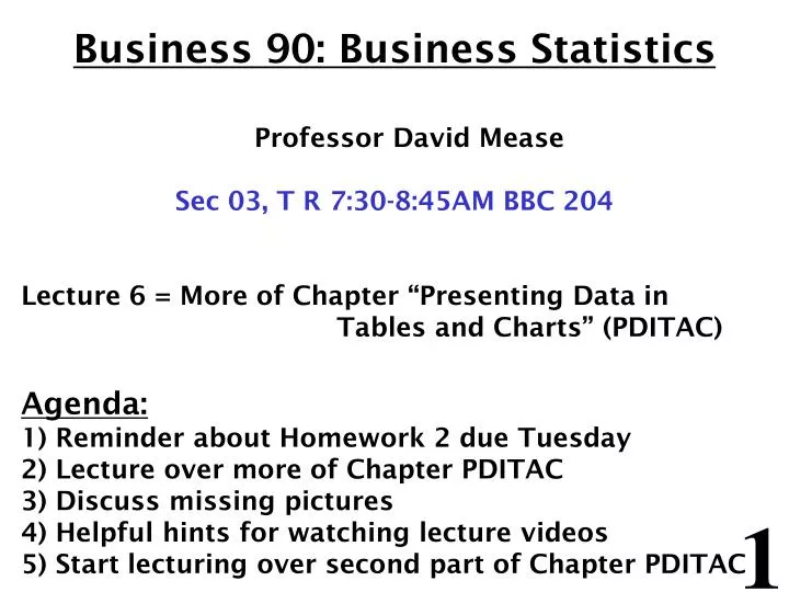
Business 90: Business Statistics Professor David Mease Sec 03, T R7:30-8:45AM BBC 204 Lecture 6 = More of Chapter “Presenting Data in Tables and Charts” (PDITAC) Agenda: 1) Reminder about Homework 2 due Tuesday 2) Lecture over more of Chapter PDITAC 3) Discuss missing pictures 4) Helpful hints for watching lecture videos 5) Start lecturing over second part of Chapter PDITAC
Homework 2 - Due Tuesday 2/16 1) Read the chapter entitled “Presenting Data in Tables and Charts” 2) The Excel file at http://www.cob.sjsu.edu/mease_d/old-quiz-scores.xls has Quiz 1 scores for a Bus 90 class I thought last semester. Right click this link and select "Save Target As..." to download this file onto your computer. Then open it using Excel. a) Make the frequency distribution by hand. Begin at 0 and end at 22 using 11 intervals. (Hint: You may use Excel to sort the data first if you like). b) Graph the frequency histogram by hand. c) Graph the percentage polygon by hand. d) Make the cumulative percentage distribution by hand. e) Graph the ogive by hand. f) Check your answer for part a using Excel. 3) The data at http://www.cob.sjsu.edu/mease_d/houses.xls has house prices for a sample of 1500 California homes. The prices are in thousands of dollars. Right click this link and select "Save Target As..." to download this file onto your computer. Then open it with Excel and use Excel to do the following. **Be sure to print out your solutions and bring them with you to class for the quiz.** a) Make the frequency distribution using Excel. Begin at 0 and end at 3.5 million using 7 intervals. b) Graph the percentage histogram using Excel. c) Graph the percentage polygon using Excel. d) Make the cumulative percentage distribution using Excel. e) Graph the ogive using Excel.
Statistics for Managers Using Microsoft® Excel4th Edition Presenting Data in Tables and Charts
Chapter Goals After completing this chapter, you should be able to: • Create an ordered array • Construct and interpret a frequency distribution, histogram, and polygon for numerical data • Construct and interpret a cumulative percentage distribution and ogive for numerical data • Create and interpret contingency tables, bar charts, and pie charts for categorical data • Create and interpret a scatter diagram and a least squares regression line (in other chapter p. 387-398) • Describe appropriate and inappropriate ways to display data graphically
The Cumulative Distribution The cumulative distribution lists the total percentage LESS THAN each class boundary It starts at zero and ends at 100% The corresponding polygon is called an ogive and uses the class boundaries (NOT the midpoints)
In class exercise #16: Construct a cumulative percentage distribution for the exam scores by hand.
In class exercise #17: Construct a cumulative percentage polygon (ogive) for the exam scores by hand.
Ogives in Excel These are done in Excel by “Insert” > “Chart” > “Line” and then selecting “line with markers displayed at each data value” The cumulative percents should be the “data range” Under the “series” tab at the top the “category (X) axis labels” should be your labels for the x-axis Provide a “chart title” and labels for the X axis and Y axis If you have just one line uncheck the “show legend” box under the legend tab
In class exercise #18: Construct a cumulative percentage polygon (ogive) for the exam scores using Excel.
In class exercise #18: Construct a cumulative percentage polygon (ogive) for the exam scores using Excel. ANSWER:
Missing Pictures If you were not here when I took pictures last time, please either email me a picture or have me take your picture after class sometime
You have 3 choices: 1) Watch as it loads This is done by simply clicking the link Advantage: No waiting Disadvantages: No fast forward No rewind “pause” works but “stop” ruins everything Hints for Watching Lecture Videos Using Windows Media Player
2) Download first then watch This is done by right clicking and selecting “Save Target As” Disadvantage: waiting for it to download Advantages: fast forward and rewind work “pause” and “stop” work Hints for Watching Lecture Videos Using Windows Media Player
3) Start watching but then decide to download half way through This is done by selecting “Save Media As” from the “File” menu in Media Player Advantage: Don’t have to wait as long to download Hints for Watching Lecture Videos Using Windows Media Player
Tables and Charts for Categorical Data With categorical data Instead of a frequency distribution we make a summary table Instead of a histogram we make a bar chart or maybe a pie chart
Summary Table Example Summarize data by category Example: Current Investment Portfolio Investment Amount Percentage Type (in thousands $) (%) Stocks 46.5 42.27 Bonds 32.0 29.09 CD 15.5 14.09 Savings 16.0 14.55 Total110.0 100.0 (Variable is Categorical)
Bar Chart Example Current Investment Portfolio Investment Amount Percentage Type(in thousands $) (%) Stocks 46.5 42.27 Bonds 32.0 29.09 CD 15.5 14.09 Savings 16.0 14.55 Total110.0 100.0
Pie Chart Example Current Investment Portfolio Investment Amount Percentage Type(in thousands $) (%) Stocks 46.5 42.27 Bonds 32.0 29.09 CD 15.5 14.09 Savings 16.0 14.55 Total110.0 100.0 Percentages are rounded to the nearest percent Savings 15% Stocks 42% CD 14% Bonds 29%
In class exercise #19: Here are the class levels (Freshman, Sophomore etc.) for all the students in my two classes last semester. Make a summary table by hand which gives the frequency for each class level. JR JR JR SO JR JR SO SO SO JR SO FR JR JR SO FR SR JR FR FR SR JR SR JR JR FR JR JR JR SO JR JR SO SO SO SO SO SO JR JR JR SR SO SO JR FR JR JR SO JR SO SO JR SR JR SO SO SO SO SR JR SO JR FR JR JR SO JR JR JR SO JR SO FR SO JR SO SO SO SO JR SR SO FR JR SO SO
Summary Tables Using Excel To make a summary table in Excel, it is often useful to use a “Pivot Table” to count the frequencies of the different categories, especially for large datasets. This is done by selecting “Data” and then “PivotTable and PivotChart Report” and dragging the name of the column of interest into both the row and data areas under the “Layout” menu. (Be sure you name the column where you have the data first.)
In class exercise #20: Make the same summary table as in ICE #19 now using a Pivot Table in Excel.
In class exercise #20: Make the same summary table as in ICE #19 now using a Pivot Table in Excel. ANSWER:
In class exercise #21: Construct the bar chart by hand.
Bar Charts Using Excel Once you have a summary table, you can use this to make a bar chart by using “Insert” then “Chart” then “Column” and using the “Clustered Column” (the first choice). As before tell Excel data range (the counts) and the Category X-axis Labels (under “Series”). Don’t use a legend unless you are doing multiple groups (which we aren’t now). Important – don’t try to use the numbers straight from the Pivot Table – paste them somewhere else first and then use them
In class exercise #22: Construct the same bar chart using Excel.
In class exercise #22: Construct the same bar chart using Excel. ANSWER:
Pareto Diagram • Used to portray categorical data • A bar chart, where categories are shown in descending order of frequency • A cumulative polygon is often shown in the same graph (but we won’t do this part) • Used to separate the “vital few” from the “trivial many” (=“Pareto Principal”)
Pareto Diagram Example Current Investment Portfolio % invested in each category (bar graph) cumulative % invested (line graph)
In class exercise #23: Construct the Pareto Diagram for class level using Excel.
In class exercise #23: Construct the Pareto Diagram for class level using Excel. ANSWER: