Download
1 / 17
170 likes | 550 Views
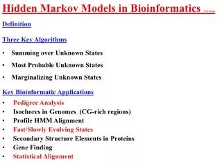
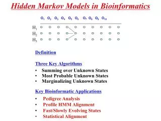
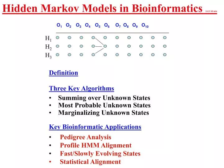
Hidden Markov Models in Bioinformatics 14.11 60 min. O 1 O 2 O 3 O 4 O 5 O 6 O 7 O 8 O 9 O 10. H 1. H 2. H 3. Definition Three Key Algorithms Summing over Unknown States Most Probable Unknown States Marginalizing Unknown States Key Bioinformatic Applications

E N D
Hidden Markov Models in Bioinformatics 14.11 60 min O1 O2O3 O4O5 O6O7 O8 O9 O10 H1 H2 H3 • Definition • Three Key Algorithms • Summing over Unknown States • Most Probable Unknown States • Marginalizing Unknown States • Key Bioinformatic Applications • Pedigree Analysis • Profile HMM Alignment • Fast/Slowly Evolving States • Statistical Alignment
Hidden Markov Models • (O1,H1), (O2,H2),……. (On,Hn) is a sequence of stochastic variables with 2 components - one that is observed (Oi) and one that is hidden (Hi). • The distribution of Ok only depends on the value of Hi and is called the emit function O1 O2O3 O4O5 O6O7 O8 O9 O10 H1 H2 H3 • The marginal distribution of the Hi’s are described by a Homogenous Markov Chain: • pi,j = P(Hk=i,Hk+1=j) • Let pi =P{H1=i) - often pi is the equilibrium distribution of the Markov Chain. • Conditional on Hk (all k), the Ok are independent.
What is the probability of the data? The probability of the observed is , which could be hard to calculate. However, these calculations can be considerably accelerated. Let the probability of the observations (O1,..Ok) conditional on Hk=j. Following recursion will be obeyed: O1 O2O3 O4O5 O6O7 O8 O9 O10 H1 H2 H3
Let be the sequences of hidden states in the most probably hidden path ie ArgMaxH[ ]. Let be the probability of the most probable path up to k ending in hidden state j. The actual sequence of hidden states can be found recursively by O1 O2O3 O4O5 O6O7 O8 O9 O10 H1 H2 H3 What is the most probable ”hidden” configuration? Again recursions can be found:
What is the probability of specific ”hidden” state? Let be the probability of the observations from k+1 to n given Hk=j. These will also obey recursions: The probability of the observations and a specific hidden state can found as: And of a specific hidden state can found as: O1 O2O3 O4O5 O6O7 O8 O9 O10 H1 H2 H3
O1 O2O3 O4O5 O6O7 O8 O9 O10 H1 H2 H3 Baum-Welch, Parameter Estimation or Training Objective: Evaluate Transition and Emission Probabilities • Set pij and e( ) arbirarily to non-zero values • Use forward-backward to re-evaluate pij and e( ) • Do this until no significant increase in probability of data To avoid zero probabilities, add pseudo-counts. Other numerical optimization algorithms can be applied.
positions 1 n 1 sequences k slow - rs HMM: fast - rf Likelihood Recursions: Likelihood Initialisations: Fast/Slowly Evolving States Felsenstein & Churchill, 1996 • pr - equilibrium distribution of hidden states (rates) at first position • pi,j - transition probabilities between hidden states • L(j,r) - likelihood for j’th column given rate r. • L(j,r) - likelihood for first j columns given j’th column has rate r.
Data 1 2 3 Trees T 1 2 i-1 i L Recombination HMMs
Statistical Alignment Steel and Hein,2001 + Holmes and Bruno,2001 T An HMM Generating Alignments - # # E # # - E * * lb l/m (1- lb)e-m l/m (1- lb)(1- e-m) (1- l/m) (1- lb) - # lb l/m (1- lb)e-m l/m (1- lb)(1- e-m) (1- l/m) (1- lb) _ #lb l/m (1- lb)e-m l/m (1- lb)(1- e-m) (1- l/m) (1- lb) # - lb C C A C Emit functions: e(##)= p(N1)f(N1,N2) e(#-)= p(N1),e(-#)= p(N2) p(N1) - equilibrium prob. of N f(N1,N2) - prob. that N1 evolves into N2
Elston-Stewart (1971) -Temporal Peeling Algorithm: Father Mother Condition on parental states Recombination and mutation are Markovian Lander-Green (1987) - Genotype Scanning Algorithm: Father Mother Condition on paternal/maternal inheritance Recombination and mutation are Markovian Comment: Obvious parallel to Wiuf-Hein99 reformulation of Hudson’s 1983 algorithm Probability of Data given a pedigree.
Further Examples poor HMM: rich Isochore: Churchill,1989,92 Lp(C)=Lp(G)=0.1, Lp(A)=Lp(T)=0.4, Lr(C)=Lr(G)=0.4, Lr(A)=Lr(T)=0.1 Likelihood Recursions: Likelihood Initialisations: Simple Eukaryotic Gene Finding: Burge and Karlin, 1996 Simple Prokaryotic
Secondary Structure Elements: Goldman, 1996 Further Examples L L L a a HMM for SSEs: Adding Evolution: SSE Prediction: Profile HMM Alignment: Krogh et al.,1994
Summary O1 O2O3 O4O5 O6O7 O8 O9 O10 H1 H2 H3 • Definition • Three Key Algorithms • Summing over Unknown States • Most Probable Unknown States • Marginalizing Unknown States • Key Bioinformatic Applications • Pedigree Analysis • Isochores in Genomes (CG-rich regions) • Profile HMM Alignment • Fast/Slowly Evolving States • Secondary Structure Elements in Proteins • Gene Finding • Statistical Alignment
& Variables: Ordinary letters: • A starting symbol: ii. A set of substitution rules applied to variables in the present string: Regular Context Free Context Sensitive General (also erasing) finished – no variables Grammars: Finite Set of Rules for Generating Strings
Simple String Generators Terminals(capital)---Non-Terminals(small) i. Start with SS --> aTbS T --> aSbT One sentence – odd # of a’s: S-> aT -> aaS –> aabS -> aabaT -> aaba ii. S--> aSabSbaa bb One sentence (even length palindromes): S--> aSa --> abSba --> abaaba
Stochastic Grammars The grammars above classify all string as belonging to the language or not. All variables has a finite set of substitution rules. Assigning probabilities to the use of each rule will assign probabilities to the strings in the language. If there is a 1-1 derivation (creation) of a string, the probability of a string can be obtained as the product probability of the applied rules. i. Start with S.S --> (0.3)aT (0.7)bS T --> (0.2)aS (0.4)bT (0.2) *0.2 *0.7 *0.3 *0.3 *0.2 S -> aT -> aaS –> aabS -> aabaT -> aaba ii. S--> (0.3)aSa (0.5)bSb (0.1)aa (0.1)bb *0.1 *0.3 *0.5 S -> aSa -> abSba -> abaaba
Recommended Literature Vineet Bafna and Daniel H. Huson (2000) The Conserved Exon Method for Gene Finding ISMB 2000 pp. 3-12 S.Batzoglou et al.(2000) Human and Mouse Gene Structure: Comparative Analysis and Application to Exon Prediction. Genome Research. 10.950-58. Blayo, Rouze & Sagot (2002) ”Orphan Gene Finding - An exon assembly approach” J.Comp.Biol. Delcher, AL et al.(1998) Alignment of Whole Genomes Nuc.Ac.Res. 27.11.2369-76. Gravely, BR (2001) Alternative Splicing: increasing diversity in the proteomic world. TIGS 17.2.100- Guigo, R.et al.(2000) An Assesment of Gene Prediction Accuracy in Large DNA Sequences. Genome Research 10.1631-42 Kan, Z. Et al. (2001) Gene Structure Prediction and Alternative Splicing Using Genomically Aligned ESTs Genome Research 11.889-900. Ian Korf et al.(2001) Integrating genomic homology into gene structure prediction. Bioinformatics vol17.Suppl.1 pages 140-148 Tejs Scharling (2001) Gene-identification using sequence comparison. Aarhus University JS Pedersen (2001) Progress Report: Comparative Gene Finding. Aarhus University Reese,MG et al.(2000) Genome Annotation Assessment in Drosophila melanogaster Genome Research 10.483-501. Stein,L.(2001) Genome Annotation: From Sequence to Biology. Nature Reviews Genetics 2.493-