Download
1 / 35
360 likes | 555 Views
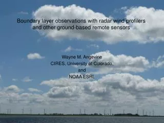
Boundary layer observations with radar wind profilers and other ground-based remote sensors. Wayne M. Angevine CIRES, University of Colorado, and NOAA ESRL. Outline. Wind profiler Principles of operation Quantities measured Time & height resolution Uncertainties

E N D
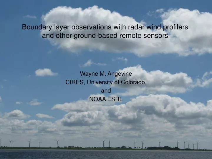
Boundary layer observations with radar wind profilers and other ground-based remote sensors Wayne M. Angevine CIRES, University of Colorado, and NOAA ESRL
Outline • Wind profiler • Principles of operation • Quantities measured • Time & height resolution • Uncertainties • Other ground-based remote sensors • Lidars • Sodars • Applications • Air quality • Weather forecasting / modeling • Science examples • Assimilation into mesoscale models • Morning transition • Entrainment • Afternoon transition • Coastal flows • Diurnal / slope flows • Thermal structure (statistics by lidar)
What’s a profiler? • Properly “radar wind profiler” • Sensitive Doppler radar • Vertical beam and 2-4 beams at 15-20° off vertical • Low power, long dwell time, and low cost compared to weather radars • Return signal is Bragg scattered from refractivity variations in clear air • Any hydrometeors or insects may contribute or even dominate • Range depends on frequency • BL profilers are at UHF (typically ~1 GHz) • Radio acoustic sounding (RASS) attachment for temperature profiling
Doppler Beam Swinging vs Spaced Antenna Doppler shift along 3 or 5 beam directions to measure winds 10 – 30 minute wind measurement Traces backscattered signal motions over 3 or 4 receivers 1 – 10 minute wind measurement Source: Bill Brown NCAR
Performance of a typical BL profiler • Wind measurement time 10 – 60 min • Height resolution 60 – 200 m • Minimum range 120 m • Max range: at least to BL top • Wind component precision ~1 m/s • May be better but no way to prove it • Careful QA required: • Low signal • Birds • Hydrometeors
What data does a profiler produce? • Winds • from radial Doppler velocities • Reflectivity • in clear air: product of humidity gradient and turbulence intensity • in precipitation: dominated by hydrometeor scattering • insects: 10 microbugs = typical clear air reflectivity • Spectral width • a measure of velocity distribution in the sample volume • in clear air: turbulence intensity (qualitative) • in precipitation: information about size distribution and/or turbulence
Example of a Precipitating Cloud System Passing over a Profiler during TEFLUN B Horizontal Axis: Time – 6 hours Vertical Axis: Altitude – 11 km Data are collected: Every minute 30 second dwell 100 meter vertical resolution (actual-105m) Courtesy of Ken Gage
Other ground-based remote sensors • Lidar and Sodar use principles similar to radar • Many types of lidars exist • Lidars provide: • very fine resolution • fast sampling • measurements of water vapor, ozone, particulate characteristics (some types) • Lidar disadvantages: • cost (capital and operational) • limited by cloud • Sodar advantages: • low cost • low minimum range • Sodar disadvantages: • noise pollution • impacted by ambient noise (including wind and rain) • low maximum range
Applications • Weather analysis & forecasting • Air quality (non-weather analysis and forecasting) • Process studies
Current Profiler Displays on AWIPS Time-Height Section of Hourly Data Isobaric Map of Hourly Data Perspective Wind Profile Display Source: Steve Koch, FSL
Assimilating profiler data into a mesoscale model for process studies • How often does a sea breeze occur in the simulation AND measurement? • Definition: Northerly component >1 m/s between 0600 and 1200 UTC and southerly >1 m/s after 1200 UTC • Assimilating 1 profiler with FDDA • WRF at 5 km grid for Houston • FDDA or FDDA+1hSST run closer to measurement at all 7 sites (at least a little) • Results not sensitive to threshold Red is FDDA run Blue has FDDA, 1-h SST, and reduced soil moisture Green has reduced soil moisture only
Coastal winds • Pease is on the mainland • Appledore is on an island ~10 km offshore • Coastline oriented northwest-southeast locally • Low-level jet stronger offshore early • Sea breeze in afternoon
Atmospheric Boundary LayerDiurnal Variation 2000 1500 1000 500 0 Inversion Convective Mixed Layer Height(meters) Residual Layer Residual Layer Stable (nocturnal) Layer Stable (nocturnal) Layer Sunrise Noon Sunrise Sunset Adapted from Introduction to Boundary Layer Meteorology -R.B. Stull, 1988
How does a profiler see the ABL? • Reflectivity is roughly the product of humidity gradient and turbulence intensity
Coastal BL with sea breeze • Pease day 215 2002
Marine BL • Appledore day 181 2002
Overcast and rain • Pease day 196 2002
Spatial variation of BL height • Urban dome or urban heat island measured by profilers in urban core and in surrounding rural areas • Implications for pollutant concentration and transport
Lidar time-height cross-sections of w with the same time scale comparing a day with light wind (top: U = 2.2 m/s) with moderate wind (bottom: U = 7.2 m/s). Courtesy of Don Lenschow
Lidar time-height cross- sections of w with the same aspect ratio (AR ≈ 7.8) comparing a day with light winds (top: U = 2.2 m/s) with moderate wind (bottom: U = 7.2 m/s).Courtesy of Don Lenschow
Time-height cross-section of w for 16 August 2996 with U = 2.2 m/s and AR ≈ 1.0 Courtesy of Don Lenschow
Morning and evening transitions and BL top entrainment • Truly stationary BLs are unusual • Transitions are critical for air quality and dispersion applications • Temporal transitions may cast light on spatial (e.g. coastal) transitions • Entrainment is poorly characterized • Profiler (and lidar) data provide a BL-top perspective to supplement more traditional in-situ surface or tower viewpoints
Morning transition • Establishes initial conditions for ABL growth • Prognostics require initialization • Models must be calibrated and validated • Profiler observations provide estimate of end of transition (onset of daytime convective ABL) • Data from two sites • Tower observations from Cabauw provide detailed insights • Long profiler and surface flux dataset from Flatland (Illinois)
Timing of transition events (composite median)
Entrainment • Definition: Incorporation of air from the free troposphere into the turbulent (convective) ABL • A change of condition (laminar to turbulent) but not necessarily of position • One of the two largest terms in the ABL heat and moisture budgets • Poorly understood and crudely parameterized • Difficult to measure
Entrainment from heat budget Entrainment flux = – heat storage + surface flux + radiative heating – advection Entrainment ratio = – entrainment flux / surface flux Measurements during Flatland (Illinois) experiments • ABL depth from profiler reflectivity (3 profilers) • Temperature change from RASS (BL average) • Surface flux from 3 Flux-PAM stations (NCAR) • Radiative heating from radiation model + aerosol measurements • Advection from Eta model
Heat budget results (mean of all good hours) zi Entrainment flux Partitioning -0.050.01 K m s-1 Fraction of total heating rate Radiative heating 0.030.002 K m s-1 Advection? 0.0010.005 K m s-1 0.100.004 K m s-1 Surface flux
Afternoon transition • Transition between fully-developed daytime convective ABL and nocturnal ABL • How does turbulence vary with time and height in the afternoon? • Sudden collapse or a gradual decline? • When does transition start? • Timing and shape of transition are critical to initiation of inertial oscillation / low-level jet, nighttime transport, distribution of pollutants, etc. • Unforced transition – all budget terms are important, few simplifications are possible • Measurements from Flatland profiler • Simple homogeneous terrain
Profiler reflectivity and spectral width patterns for a “typical” day Doppler spectral width
When does transition start? • Three different definitions based near daytime max. ABL height • All definitions show transition starting well before sunset sunset
Final thoughts • Ground-based remote sensors provide continous data in a column or volume • a valuable complement to sparse aircraft measurements • Can be (and usually should be) deployed in groups • Wind profilers are good for much more than just wind • Output must be used carefully – beware of “black boxes”
References (1) Angevine, W.M., A.B. White, and S.K. Avery, 1994: Boundary layer depth and entrainment zone characterization with a boundary layer profiler. Boundary Layer Meteor., 68, 375-385. Angevine, W.M., and J.I. MacPherson, 1995: Comparison of wind profiler and aircraft wind measurements at Chebogue Point, Nova Scotia. J. Atmos. Oceanic Technol., 12, 421-426. Carter, D.A., K.S. Gage, W.L. Ecklund, W.M. Angevine, P.E. Johnston, A.C. Riddle, J. Wilson, and C.R. Williams, 1995: Developments in UHF lower tropospheric wind profiling at NOAA's Aeronomy Laboratory. Radio Sci., 30, 977-1001. Riddle, A.C., W.M. Angevine, W.L. Ecklund, E.R. Miller, D.B. Parsons, D.A. Carter, and K.S. Gage, 1996: In situ and remotely sensed horizontal winds and temperature intercomparisons obtained using Integrated Sounding Systems during TOGA COARE. Contributions to Atmospheric Physics, 69, 49-62. Angevine, W.M., 1997: Errors in mean vertical velocities measured by boundary layer wind profilers. J. Atmos. Oceanic. Technol., 14, 565-569. Angevine, W.M., P.S. Bakwin, and K.J. Davis, 1998: Wind profiler and RASS measurements compared with measurements from a 450 m tall tower. J. Atmos. Oceanic. Technol., 15, 818-825. Grimsdell, A.W., and W.M. Angevine, 1998: Convective boundary layer height measured with wind profilers and compared to cloud base. J. Atmos. Oceanic Technol., 15, 1332-1339. Angevine, W.M., 1999: Entrainment results including advection and case studies from the Flatland boundary layer experiments. J. Geophys. Res., 104, 30947-30963.
References (2) Cohn, S.A., and W.M. Angevine, 2000: Boundary layer height and entrainment zone thickness measured by lidars and wind profiling radars. J. Appl. Meteorol., 39, 1233-1247. Angevine, W.M., and K. Mitchell, 2001: Evaluation of the NCEP mesoscale Eta model convective boundary layer for air quality applications. Mon. Wea. Rev., 129, 2761-2775. Angevine, W.M., H. Klein Baltink, and F.C. Bosveld, 2001: Observations of the morning transition of the convective boundary layer. Boundary-Layer Meteorol., 101, 209-227. Grimsdell, A.W., and W.M. Angevine, 2002: Observations of the afternoon transition of the convective boundary layer. J. Appl. Meteorol., 41, 3-11. Angevine, W.M., C.J. Senff, and E.R. Westwater, 2002: Boundary Layers/Observational techniques -- Remote. Encyclopedia of Atmospheric Sciences, J.R. Holton, J. Pyle, and J.A. Curry, Eds., Academic Press, 271-279. Angevine, W.M., A.B. White, C.J. Senff, M. Trainer, and R.M. Banta, 2003: Urban-rural contrasts in mixing height and cloudiness over Nashville in 1999. J. Geophys. Res., 108(D3), doi:10.1029/2001JD001061. Nielsen-Gammon, J.W., R.T. McNider, W.M. Angevine, A.B. White, and K. Knupp, 2007: Mesoscale model performance with assimilation of wind profiler data: Sensitivity to assimilation parameters and network configuration. J. Geophys. Res., 112, D09121, doi:10.1029/2006JD007633. Angevine, W.M., 2008: Transitional, entraining, cloudy, and coastal boundary layers. Acta Geophysica, 56, 2-20.
Acknowledgements • Ken Gage, Don Lenschow for slides