Download
1 / 34

E N D
Classical mechanics era: 1687 - Newton's mechanics 1788 - Lagrange's mechanics 1834 Hamiltonian mechanics 1864 - Maxwell's equations 1900 – blotzmann equation • At the end of the nineteenth century physics was thought essentially consists of: • classical mechanics • the theory of electromagnetism • thermodynamics • And this was the main success of classical physics who made people believe that the ultimate description of the nature had been achieved. • But at the beginning of the twentieth century, however, classical physics, which had been quite unassailable. introduction
Two major fronts • Relativistic mechanics: • Einstein in 1905 showed in his special theory of relativity that the validity of Newtonian mechanics ceases at very high speeds. • Microscopic domain: • atomic and subatomic structure , black body radiation, photo electriceffect ,Compton effect ,pair production,atomic stability and atomic spectroscopy etc .
Quantum mechanics The failure of classical mechanics to explain the above Phenomenas give rise to the birth of new theory called “ Quantum mechanics”. Development Era of QM
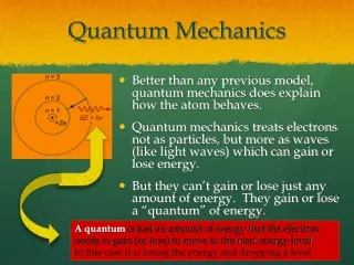
Formulation of quatum mechanics at beginning: • Heisenberg approach( matrix mechanics) • schrodinger approach( wave mechanics) • Quantum mechanics : • Classical mechanics is an approximation of quantum mechanics. • Classical mechanics is an approximation of quantum mechanics means we get the classical results from the quantum mechanics. • for example, that the radius of the electron's orbit in a • ground-state hydrogen atom is always exactly 5.3 x 10-'1 m, • as the Bohr theory does, quantum mechanics states that this • is the most probable radius. In a suitable experiment most • trials will yield a different value, either larger or smaller, but • the value most likely tobe found will be 5.3 X 10⁻¹¹ m.
If quantum mechanics is to be more general than classical mechanics, it must contain classical mechanics as a limiting case and this can be illustrated by Ehrenfest theorem, • “ eqution of motion in classical is same is that of expectation value equation in quantum mechanics.” • d\dt<r>=1/m<p> • d\dt<p>=-<del(v)>
these two equations certainly establish a connection between quantum mechanics and classical mechanics. • Question:How does one decide on when to use classical or quantum mechanics to describe the motion of a given system? • The answer is by comparing the size of those quantities of the system that have the dimensions of an action with the Planck constant h, . • But if the value of the action of a system is too large compared to h then this system can be accurately described by classical physics.
Wave function • To describe a system in quantum mechanics, we use a mathematical entity (a complex function) belonging to a Hilbert space, the state vector Ѱ(x,t) which contains all the information we need to know about the system and from which all needed physical quantities can be computed. • It is noted that “Ѱ” itself has no physicl significance , but the absolute magnitude ||^2 evaluated at a particular time and place tells us the probability of finding the system represented by in that (x, y, z, t) state.
It is noted the state vector can be represented by two ways ; • Ѱ(x,t) • |Ѱ(x,t)> , <Ѱ(x,t)| • to describe the state of a one-dimensional particle in quantum mechanics we use a complex function Ѱ(x,t) instead of two real real numbers (x, p) in classical physics. • for example the wave function of a particle moving • along x axis is, • Ѱ(x,t)=expi(kx –wt)
NORMALIZATION • It is noted that in quantum mechanics we cannot predict the exact position of the particle rather we find the probability density in a given region of space. • let the probability of finding the particle represented by Ѱ between position x1 & x2 at time t is given by • If • probability = 1 ( max) • probability = 0 (min ) • A wave function that obey above equation is called normalized . Actually in normalization our main concerned is to find the value of constant . Probability
Example:Calculate the probability that the a measurement will find the particle represented by between x = 0 and x = 0.5.
But Here’s a plot of the probability density (magnitude of wave function squared). So we can’t say about the probability that the particle is at x = 0.5 (Heisenberg), but you can talk about the probability that the particle can be found within an incremental dx centered at x = 0.5.
Well behaved wave function • With every physical quantity we associate some mathematical object which is called eigen vector , eigen state , state vector , wave function. • Besides normalization an acceptable and well behaved wave function must • satisfy some properties given below, • must be continuous every where • must be finite every at all points • must be single valued • must be differentiable • must be square integrable
“I think that I can safely say that nobody understands quantum mechanics.”—Richard Feynman (Nobel Prize, 1965)” • THE WAVE EQUATION • I have been seen in several books that particles have wave properties, and we have seen also seen experimental verification of support this claim. • It means If particles have wave properties and can be described by a wave function ψ, there must be a wave equation for particles. Just like in classical mechanics Newtonian equation. • before developing equation we just review the wave equation:
The solution y(x,t) is a wave traveling with a speed v through space (one dimension) and time. • Partial Derivative • If F is a function of (xyz), then when you take F/x, you treat y and z as constants: • to calculate 2nd order partial derivative as occur in wave equation we again differentiate it =2yz (which is the solution of the above quation) Solution of wave equation for any kind of wave has form,
The - sign represents waves traveling in the +x direction. • The + sign represents waves traveling in the -x direction. An example of a solution of the wave equation is the wave equivalent to a free particle Here it is noted that we only concerned with the real which the amplitude of the wave and discarded the imaginary part because of the general wave formula
Here it is noted that we have only concerned with the real part, which the amplitude of the wave and discarded the imaginary part because of the general wave formula
verify that is the solution of wave equation. solution:
so we conclude y=exp(i(kx-wt)) is the solution of the wave equation.
Schrödinger's Equation: Time-Dependent Form • In quantum mechanics the wave function ψ corresponds to the wave variable y , however ψ unlike y, is not itself a measurable quantity and may therefore be complex. Schrödinger's Equation: Time-Dependent Form
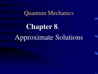
It is noted that , • We have “justified” Schrödinger's equation, but not derived it. • Just like we never derive Newton’s laws either. We justify them, show that they work, and use them. We believe them because they describe reality • The same holds for Schrödinger's equation. It is a postulated first principle, arrived at by observation of physical reality, and believed in because it successfully describes the universe.
Schrödinger’s equation has been used to explain the previously unexplainable and predict the previously unthought. If you want to replace Schrödinger’s equation with something else, the “something else” must do everything Schrödinger’s equation does, and more
Linearity and Superposition Linearity and Superposition Wave function adds, not probabilities
P2 Interference terms! Waves interfere!
it is noted that the two terms at the right hand side of this represent the difference between fig.5.2d and e and are responsible for the oscillations of the electron intensity at the screen. In sec 6.8 a similar calculation will be used to investigate why a hydrogen atom emits radiation when it undergoes a transition from one quantum state to another lower enery.