Download
1 / 23
230 likes | 392 Views
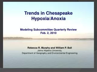
Trends in Chesapeake Hypoxia/Anoxia Modeling Subcommittee Quarterly Review Feb. 2, 2010. Rebecca R. Murphy and William P. Ball Johns Hopkins University, Department of Geography and Environmental Engineering. Outline. Chesapeake Bay Environmental Observatory (CBEO) Hypoxic volume trends

E N D
Trends in Chesapeake Hypoxia/Anoxia Modeling Subcommittee Quarterly ReviewFeb. 2, 2010 Rebecca R. Murphy and William P. Ball Johns Hopkins University, Department of Geography and Environmental Engineering
Outline • Chesapeake Bay Environmental Observatory (CBEO) • Hypoxic volume trends • Stratification trends • Statistical models • Possibility that large-scale climatic forces are affecting hypoxia/stratification • Brief comparison to model output
CBEO and Hypoxia Analysis Data Sets Chesapeake Bay Program data USGS River Monitoring Historic CBI data Model outputs etc… New Tools/Methods CBEO website: http://cbeo.communitymodeling.org investigate Generated from data in Hagy et al. (2004) in Estuaries
DO Analysis Approach: Analyze hypoxic volume with as much temporal and spatial resolution as possible • Interpolate DO and calculate hypoxic volume for each data collection cruise • Examine time series • Look at where/when changes are occurring in DO patterns
rN,vol = 0.31 (p=0.07) rN,vol = - 0.44 (p=0.006) rN,vol = 0.50 (p=0.001) rN,vol = 0.88 (p=4e-17) Data Sources: USGS, CBP
June DO: Oxygen depletion is happening earlier in summer in recent years Stratification: Plays a role in oxygen depletion Approach: • Calculate pycnocline strength • Examine time series • Identify where/when changes are occurring • Look for significant relationships between stratification and hypoxic volume trends Early July DO: More hypoxic volume than anticipated from nutrients alone Nutrients Late July DO: Hypoxic volume follows trend expected from nutrient loads
Stratification Strength Calculation Pycnocline Data Source: CBP
Stratification Strength Calculation 1. Calculate Brunt Väisälä Frequency 2. Interpolate maximum Brunt Väisälä Frequency (N2) 3. Average max N2 in region of interest Average = 0.015
Analysis: Stratification to Early July Hypoxic Volume (‘85-’09) HypoxicVolEarlyJuly = 6 + 0.8 (StratificationJune) + 2 (StratificationEarlyJuly) + e R2 = 0.74 (p=3e-07)
June DO: Oxygen depletion is happening earlier in summer in recent years Changing Climatic Forces (NAO, wind, GSI, sea level rise?) • June • Stratification: • Increasing over time • Causes less vertical mixing of oxygen Early July DO: More hypoxic volume than anticipated from nutrients alone Nutrients • July Stratification: • Not increasing over time • Very variable Climatic Forces Wind speeds much more variable year-to-year in July Late July DO: Hypoxic volume follows trend expected from nutrient loads
Possible Climatic Factors NAO • North Atlantic Oscillation • Index has been higher for last 25 years – influences mid-Atlantic climate in multiple ways • Wind direction shifts: (related to NAO) • Winds from south tend to weaken stratification Graph from Jeremy Testa (UMCES) Wind shift and possible relation to hypoxic volume identified by Malcolm Scully (Old Dominion), data=NOAA
Possible Climatic Factors: Salinity Changes • Gulf Stream Position (related to NAO) • Index has been higher for last 25 years – means saltier mid-Atlantic waters (Lee and Lwiza 2008) • Sea Level Rise • Evidence of increased Bay salinity (Hilton et al. 2008) Plymouth Marine Laboratory data NOAA data
Continuing Work • Investigation of the causes of the increase in early summer stratification and hypoxia • Expanded interpolation efforts into tributaries to examine hypoxia vs. stratification trends
Comparison to Model Output 57k output from Mark Noel March ‘09
Acknowledgements • Chesapeake Bay Environmental Observatory (CBEO) team, including: • Dr. Michael Kemp and Jeremy Testa (UMCES) • Drs. Dominic Di Toro and Damian Brady (UDel) • Dr. Randal Burns and Eric Perlman (JHU CS) • Data sources: Chesapeake Bay Institute, Chesapeake Bay Program, USGS, NOAA • NSF funding of the CBEO project
References • Guo, X. and Valle-Levinson, A. (2008). “Wind effects on the lateral structure of density-driven circulation in Chesapeake Bay.” Continental Shelf Research, 28, 2450-2471. (Univ of Florida) • Hagy, J. D., Boynton, W.R., Wood, C.W., Wood, K.V. (2004). "Hypoxia in the Chesapeake Bay, 1950-2001: long-term changes in relation to nutrient loading and river flows." Estuaries, 27(4), 634-658. • Hilton, T.W., Najjar, R.G., Zhong, L., and M. Li. (2008). “Is there a signal of sea-level rise in Chesapeake Bay salinity?” Journal of Geophysical Research, 113, C09002. (Penn State, UMCES) • Lee, Y.J. and K.M.M. Lwiza. 2008. Factors driving bottom salinity variability in the Chesapeake Bay.Continental Shelf Research 28:1352-1362. (Stony Brook) • Scully, M.E. (2009). “The importance of decadal-scale climate variability to wind-driven modulation of hypoxia in Chesapeake Bay.” Nature Precedings, Posted Jun 2, 2009. (Old Dominion) Data Sources: • CBP: http://www.chesapeakebay.net/data_waterquality.aspx • CBI and other historic data: http://archive.chesapeakebay.net/data/historicaldb/historicalmain.htm • USGS: http://va.water.usgs.gov/chesbay/RIMP/ and http://waterdata.usgs.gov/nwis/monthly/ • NCDC (wind data, Patuxent Naval Air Station: http://cdo.ncdc.noaa.gov/pls/plclimprod/poemain.accessrouter?datasetabbv=DS3505 • NOAA (sea level): http://tidesandcurrents.noaa.gov/sltrends/sltrends.shtml • GSI: http://web.pml.ac.uk/gulfstream/default.htm
Theory: Stratification and Mixing BVF BVF Richardson Number, Ri (Ri: balance between buoyant and shear forces) vertical velocity gradient Ri Vertical Diffusivity, Ez (Munk and Anderson 1948) Ez,0 = Eddy diffusivity with no stratification a,b = coefficients