Download

1 / 24
240 likes | 398 Views
Stochastic Evaluation of the 1st Axxom Case Study. Holger Hermanns Yaroslav S. Usenko (Saarbrücken & Twente) (Twente) with contributions of Henrik Bohnenkamp, Joost-Pieter Katoen, Angelika Mader (Twente).

E N D
Stochastic Evaluation of the 1st Axxom Case Study Holger Hermanns Yaroslav S. Usenko (Saarbrücken & Twente) (Twente) with contributions of Henrik Bohnenkamp, Joost-Pieter Katoen, Angelika Mader (Twente)
Performance & Availability Factors • Availabability factor: • reflects the fraction of time the machine is operational. • only used if no model of operation hours is available. • An availability factor of 0.8 extends the occupation times used for planning by a factor of 1/0.8, i.e., 1.25. A six-hour disperser job is scheduled for 14 hours • Performance factor: • reflects unpredictable perturbations of the production process. • A performance factor of 0.8 extends the occupation times used for planning by a factor of 1/0.8, i.e., 1.25.
Our View • Both the performance and the availability factors relate to unplanned or unplannable pertubations of the production process. • They reflect random influences with partially known characteristics. • This holds in particular for the performance factor, and to a lesser extent for the availability factor.
Behaviour of a single machine Anticipated behaviour: 0 6 14 20 28 34 42 48 56 Risk: 0 6 14 20 28 34 42 48 56 Scheduled behaviour: 0 6 14 20 28 34 42 48 56
Our Approach • Develop a model reflecting the stochastic perturbations. • Use this model to study a-priori computed valid schedules. • Quantify the risk • to violate the schedule, and • to miss deadlines. • Note: different valid schedules may differ w.r.t. these risks. • This provides means to rankvalid schedules. • We exercise this approach using Modest.
Semantics of MoDeST: STA, ‘stochastic timed automata’, a model made up from timed automata with deadlines [Alur/Dill, Bornot/Sifakis] stochastic automata [D’Argenio/Brinksma/Katoen] probabilistic automata [Segala/Lynch] MoDeST (1) cash • A specification formalism for Modelling and Description of Stochastic Timed sytems cash set_price w(y120) u(y240) tau y:=0 get_prod no_price
MoDeST (2): syntax cash cash set_price w(y120) u(y240) tau y:=0 get_prod no_price xd:=U[10,20] x:=0 u(xxd) w(xxd)
A schedule, produced by A. Mader a task a job machines deadline job types • 29 jobs, grouped into 3 job types, • each job type is composed of multiple partially concurrent tasks, • running on 11 different ‘machines’. • each job has a deadline of 336 hrs (2 weeks)
Machines in Modest work (amount,deadline) idle missed br:=Random(...) w:=0 [w=br && br < amount] [cjobs > deadline] done work [amount < br && w = amount] break br:=Random(...) rep := Random(...) y:= 0 amount -= br fix down [y=rep] process TP2_machine() // Disperser { clock w,y; float br,r,work,deadline; do{:: when (TP2_work>0) act_work_TP2 {= work=TP2_work, TP2_work=0, deadline=TP2_deadline, w=0, //current working time br=Rand(...) //next time to break =}; do { :: when (cjobs>=deadline) act_error_TP2 {= TP2_done=2 =}; break :: when (br>=work && w>=work) act_done_TP2 {= TP2_done=1 =}; break :: when (br<work && w>=br) act_break_TP2 {= work-=br, r=Rand(...), y=0 =}; when(y==r) act_repaired_TP2 {= w=0, br=Rand(...) =} } } }
Jobs (type 2) process Job_type2(int number, float starttime, float earliesttime, float deadline) { int mv=0,ds=0; // which mixing vessel and dose spinner will we get? clock c; when(cjobs==starttime) tau {= ii+=1 =}; // starting time according to the schedule // disperser for 27 when(TP2_lock==0) tau {= TP2_lock=1, TP2_deadline=deadline-49-26-2, TP2_work=27 =}; when(TP2_done>0) tau {= TP2_done=0, TP2_lock=0 =}; // Lock an UNI mixing vessel alt{ :: when(MVU1_lock==0) tau {= mv=1, MVU1_lock=1 =} :: when(MVU2_lock==0) tau {= mv=2, MVU2_lock=1 =} }; // Two parallel activities: par{... }; ... // are we on time? alt{ :: when(cjobs<=deadline) tau {= d+=1, dd+=1 =} ; INC_j(number) :: when(cjobs>deadline) tau } }
Schedule violations vs. deadline misses recover from schedule violations: allow tasks to happen later than scheduled, unless job deadline miss is for sure. profit from slack in schedules: allow tasks to grab machines as early as possible, respecting scheduled order (not timing). schedule violation risk: It seems wise to
The system par{ :: ABF1_machine() :: ABF2_machine() :: TP2_machine() :: DOK1_machine() :: DOK2_machine() :: DVT1_machine( :: BR1_machine() :: HDL1_machine() :: MVU1_machine() :: MVU2_machine() :: MVM1_machine() :: MVM2_machine() :: MVM3_machine() :: do {:: tau {= i+=1, d=0, cjobs=0 =}; par{ :: Job_type1(17, js17, 101, 101+336) :: Job_type2(15, js15, 52, 52+336) :: Job_type2( 5, js5, 191, 191+336) :: Job_type2(14, js14, 274, 274+336) :: Job_type2(18, js18, 278, 278+336) :: Job_type2( 4, js4, 388, 388+336) :: Job_type3(28, js28, 276, 276+336) }; INC_d(d) } }
It is natural to interpret the availability/performance factor as the ratio of time the system is available/performing. In the dependability context this ratio arises as: So a factor of, say, 0.8 relates MTBF and MTTR: If MTBF and MTTR are given, the best probabilistic approx- imation is obtained with negative exponential distributions, para- metrized with these mean durations. Unfortunately, the means are not given, only their ratio. Intermezzo: Stochastic Perturbations Mean time between failures Mean time to repair
MOTOR Other tools’ outputs APNN E MC2 Prism CADP Mobius T Uppaal TorX CADP Spin Rapture PrUppaal Prism MoDeST compiler Discrete event simulator
What we considered Caution: Unfair comparison A six-hour disperser job scheduled for 14 hours but not in these schedules
Some comparative results Job success probability
Some comparative results Job success probability “pace”
Conclusion • Stochastic machine model for 1st Axxom case. • Allows ranking of schedules. • Provides deeper insight into schedule particularities. • Depends on more than just the perf./avail. factors. • Motor is an early prototype. First (semi-)serious application.
Perspective UPPAAL 1995 - 2000 • Well, at least Motor has quite some potential for a similar improvement in the next decade. 1994 1995 Every 9 month 10 times better 1996 performance! 1997 1998 1999 2k Dec’96 Sep’98 b 9 Kim G. Larsen