Beginning Programming for Engineers
Explore the fundamentals of symbolic mathematics and learn how to leverage MATLAB's Symbolic Toolbox for various mathematical operations. This toolbox enables engineers and scientists to manipulate algebraic expressions, solve equations, and perform calculus operations like differentiation and integration. Discover how to create and substitute symbolic variables, use MATLAB to define, solve algebraic and differential equations, and visualize symbolic expressions. This guide is ideal for those looking to enhance their programming skills in engineering applications.

Beginning Programming for Engineers
E N D
Presentation Transcript
Beginning Programming for Engineers Symbolic Math Toolbox
What is Symbolic Math? Symbolic mathematics deals with equations before you plug in the numbers. • Calculus – integration, differentiation, Taylor series expansion, … • Linear Algebra – inverses, determinants, eigenvalues, … • Simplification – algebraic and trigonometric expressions • Equation Solutions – algebraic and differential equations • Transforms – Fourier, Laplace, Z transforms and inverse transforms, …
Matlab's Symbolic Toolbox • The Symbolic Toolbox allows one to use Matlab for symbolic math calculations. • The Symbolic Toolbox is a separately licensed option for Matlab. (The license server separately counts usage of the Symbolic Toolbox.) • Recent versions use a symbolic computation engine called MuPAD. Older versions used Maple. Matlab translates the commands you use to work with the appropriate engine. • One could also use Maple or Mathematica for symbolic math calculations. • Strategy: Use the symbolic toolbox only to develop the equations you will need. Then use those equations with non-symbolic Matlab to implement your program.
Symbolic Objects Use sym to create a symbolic number, and double to convert to a normal number. • >> sqrt(2) • ans = 1.4142 • >> var = sqrt(sym(2)) • var = 2^(1/2) • >> double(var) • ans = 1.4142 • >> sym(2)/sym(5) + sym(1)/sym(3) • ans = 11/15
Symbolic variables Use syms to define symbolic variables. (Or use sym to create an abbreviated symbol name.) • >> syms m n b c x • >> th = sym('theta') • >> sin(th)ans = sin(theta) • >> sin(th)^2 + cos(th)^2ans = cos(theta)^2 + sin(theta)^2 • >> y = m*x + by = b + m*x
Substituting into symbolic expressions The subs function substitutes values or expressions for variables in a symbolic expression. • >> clear>> syms m x b>> y = m*x + b → y = b + m*x • >> subs(y,x,3) → ans = b + 3*m • >> subs(y, [m b], [2 3]) → ans = 2*x + 3 • >> subs(y, [b m x], [3 2 4])→ ans = 11 The symbolic expression itself is unchanged. • >> y →y = b + m*x
Substitutions, continued Variables can hold symbolic expressions. • >> syms th z>> f = cos(th) → f = cos(th)>> subs(f,pi) → ans = -1 Expressions can be substituted into variables. • >> subs(f, z*pi) → ans = cos(pi*z)
Differentiation Use diff to do symbolic differentiation. >> clear>> syms m x b th n y >> y = m*x + b;>> diff(y, x) → ans = m>> diff(y, b) → ans = 1 >> p = sin(th)^n → p = sin(th)^n>> diff(p, th) → ans = n*cos(th)*sin(th)^(n - 1)
Integration >> clear>> syms m b x>> y = m*x + b; Indefinite integrals >> int(y, x) → ans = (m*x^2)/2 + b*x>> int(y, b) → ans = (b + m*x)^2/2>> int(1/(1+x^2)) → ans = atan(x) Definite integrals >> int(y,x,2,5) → ans = 3*b + (21*m)/2>> int(1/(1+x^2),x,0,1) → ans = pi/4
Solving algebraic equations >> clear>> syms a b c d x>> solve('a*x^2 + b*x + c = 0') → ans = % Quadratic equation! -(b + (b^2 - 4*a*c)^(1/2))/(2*a) -(b - (b^2 - 4*a*c)^(1/2))/(2*a)>> solve('a*x^3 + b*x^2 + c*x + d = 0') → Nasty-looking expression >> pretty(ans) → Debatable better-looking expression From in-class 2: >> solve('m*x + b - (n*x + c)', 'x') → ans = -(b - c)/(m - n)>> solve('m*x + b - (n*x + c)', 'b') → ans = c - m*x + n*x>> collect(ans, 'x') → ans = c - x*(m - n)
Solving systems of equations Systems of equations can be solved. • >> [x, y] = solve('x^2 + x*y + y = 3', ... • 'x^2 - 4*x + 3 = 0') → Two solutions: x = [ 1 ; 3 ] • y = [ 1 ; -3/2 ] • >> [x, y] = solve('m*x + b = y', 'y = n*x + c') • → Unique solution: x = -(b - c)/(m - n) • y = -(b*n - c*m)/(m - n) If there is no analytic solution, a numeric solution is attempted. • >> [x,y] = solve('sin(x+y) - exp(x)*y = 0', ... • 'x^2 - y = 2') → x = -0.66870120500236202933135901833637 y = -1.5528386984283889912797441811191
Plotting symbolic expressions The ezplot function will plot symbolic expressions. • >> clear; syms x y>> ezplot( 1 / (5 + 4*cos(x)) );>> hold on; axis equal>> g = x^2 + y^2 - 3; • >> ezplot(g);
More symbolic plotting >> clear; syms x >> digits(20) >> [x0, y0] = solve(' x^2 + y^2 - 3 = 0', ... 'y = 1 / (5 + 4*cos(x)) ') → x0 = -1.7171874987452662214 y0 = 0.22642237997374799957 >> plot(x0,y0,'o') >> hold on >> ezplot( diff( 1 / (5 + 4*cos(x)), x) )
Solving differential equations We want to solve: Use D to represent differentiation against the independent variable. • >> y = dsolve('Dy = -a*y') → y = C5/exp(a*t) Initial values can be added: • >> y = dsolve('Dy = -a*y', 'y(0) = 1') → y = 1/exp(a*t)
More differential equations Second-order ODEs can be solved: >> y = dsolve('D2y = -a^2*y', ... 'y(0) = 1, Dy(pi/a) = 0') → y = exp(a*i*t)/2 + 1/(2*exp(a*i*t)) Systems of ODEs can be solved: >> [x,y] = dsolve('Dx = y', 'Dy = -x') → x = (C13*i)/exp(i*t) - C12*i*exp(i*t) y = C12*exp(i*t) + C13/exp(i*t)
Simplifying expressions >> clear; syms th>> cos(th)^2 + sin(th)^2 → ans = cos(th)^2 + sin(th)^2>> simplify(ans) → ans = 1 >> simple(cos(th)^2 + sin(th)^2) >> [result,how] = simple(cos(th)^2 + ... sin(th)^2) → result = 1 how = simplify >> [result,how] = simple(cos(th)+i*sin(th)) → result = exp(i*th) how = rewrite(exp)