Introduction to Credibility CAS Seminar on Ratemaking Philadelphia, PA March 10-12, 2004

2. Introduction to Credibility CAS Seminar on Ratemaking Philadelphia, PA March 10-12, 2004

3. Purpose Today’s session is designed to encompass: • Credibility in the context of ratemaking • Classical and Bühlmann models • Review of variables affecting credibility • Formulas • Practical techniques for applying • Methods for increasing credibility

4. Outline • Background • Definition • Rationale • History • Methods, examples, and considerations • Limited fluctuation methods • Greatest accuracy methods • Bibliography

5. Background

6. BackgroundDefinition • Common vernacular (Webster): • “Credibility:” the state or quality of being credible • “Credible:” believable • So, “the quality of being believable” • Implies you are either credible or you are not • In actuarial circles: • Credibility is “a measure of the credence that…should be attached to a particular body of experience” -- L.H. Longley-Cook • Refers to the degree of believability; a relative concept

7. BackgroundRationale Why do we need “credibility” anyway? • P&C insurance costs, namely losses, are inherently stochastic • Observation of a result (data) yields only an estimate of the “truth” • How much can we believe our data?

8. BackgroundHistory • The CAS was founded in 1914, in part to help make rates for a new line of insurance -- Work Comp • Early pioneers: • Mowbray -- how many trials/results need to be observed before I can believe my data? • Albert Whitney -- focus was on combining existing estimates and new data to derive new estimates New Rate = Credibility*Observed Data + (1-Credibility)*Old Rate • Perryman (1932) -- how credible is my data if I have less than required for full credibility? • Bayesian views resurrected in the 40’s, 50’s, and 60’s

9. “Frequentist” Bayesian BackgroundMethods Limit the effect that random fluctuations in the data can have on an estimate Limited Fluctuation “Classical credibility” Make estimation errors as small as possible Greatest Accuracy “Least Squares Credibility” “Empirical Bayesian Credibility” Bühlmann Credibility Bühlmann-Straub Credibility

10. Limited Fluctuation Credibility

11. Limited Fluctuation CredibilityDescription • “A dependable [estimate] is one for which the probability is high, that it does not differ from the [truth] by more than an arbitrary limit.” -- Mowbray • How much data is needed for an estimate so that the credibility, Z, reflects a probability, P, of being within a tolerance, k%, of the true value?

12. Add and subtract ZE[T] regroup Limited Fluctuation CredibilityDerivation New Estimate = (Credibility)(Data) + (1- Credibility)(Previous Estimate) E2 = Z*T + (1-Z)*E1 = Z*T + ZE[T] - ZE[T] + (1-Z)*E1 = (1-Z)*E1 + ZE[T] +Z*(T - E[T]) Stability Truth Random Error

13. Limited Fluctuation CredibilityMathematical formula for Z Pr{Z(T-E[T]) < kE[T]} = P -or- Pr{T < E[T] + kE[T]/Z} = P E[T] + kE[T]/Z = E[T] + zpVar[T]1/2 (assuming T~Normally) -so- kE[T]/Z = zpVar[T]1/2  Z = kE[T]/zpVar[T]1/2

14. N = (zp/k)2 Limited Fluctuation CredibilityMathematical formula for Z (continued) • If we assume • That we are dealing with an insurance process that has Poisson frequency, and • Severity is constant or severity doesn’t matter • Then E[T] = number of claims (N), and E[T] = Var[T], so: • Solving for N (# of claims for full credibility, i.e., Z=1): Z = kE[T]/zpVar[T]1/2 becomes: Z = kE[T]1/2 /zp = kN1/2 /zp

15. Limited Fluctuation CredibilityStandards for full credibility Claim counts required for full credibility based on the previous derivation:

16. Limited Fluctuation CredibilityMathematical formula for Z – Part 2 • Relaxing the assumption that severity doesn’t matter, • let T = aggregate losses = (frequency)(severity) • then E[T] = E[N]E[S] • and Var[T] = E[N]Var[S] + E[S]2Var[N] • Plugging these values into the formula Z = kE[T]/zpVar[T]1/2 and solving for N (@ Z=1): N = (zp/k)2{Var[N]/E[N]+ Var[S]/E[S]2}

17. Limited Fluctuation CredibilityMathematical formula for Z – Part 2 (continued) N = (zp/k)2{Var[N]/E[N]+ Var[S]/E[S]2} Think of this as an adjustment factor to the full credibility standard that accounts for relaxing the assumptions about the data. This term is just the full credibility standard derived earlier The term on the left is derived from the claim frequency distribution and tends to be close to 1 (it is exactly 1 for Poisson). The term on the right is the square of the c.v. of the severity distribution and can be significant.

18. Limited Fluctuation CredibilityPartial credibility • Given a full credibility standard for a number of claims, Nfull, what is the partial credibility of a number N < Nfull? • The square root rule says: Z = (N/ Nfull)1/2 • For example, • let Nfull = 1,082, and • say we have 500 claims. Z = (500/1082)1/2 = 68%

19. Limited Fluctuation CredibilityPartial credibility (continued) Full credibility standards:

20. If the data analyzed is… A good complement is... Pure premium for a class Pure Premium for all classes Loss ratio for an individual Loss ratio for entire class risk Indicated rate change for a Indicated rate change for territory entire state Indicated rate change for Trend in loss ratio or the entire state indication for the country Limited Fluctuation CredibilityComplement of credibility Once partial credibility has been established, the complement of credibility, 1-Z, must be applied to something else. E.g.,

21. E.g., 81%(.60) + 75%(1-.60) E.g., 76.5%/75% -1 Limited Fluctuation CredibilityExample Calculate the expected loss ratios as part of an auto rate review for a given state, given that the expected loss ratio is 75%. • Data: Loss Ratio Claims 1995 67% 535 1996 77% 616 1997 79% 634 1998 77% 615 1999 86% 686 Credibility at: Weighted Indicated 1,0825,410 Loss RatioRate Change 3 year 81% 1,935 100% 60%78.6%4.8% 5 year 77% 3,086 100% 75% 76.5% 2.0%

22. Limited Fluctuation CredibilityIncreasing credibility • Per the formula, Z = (N/ Nfull)1/2 = [N/(zp/k)2]1/2 = kN1/2/zp • Credibility, Z, can be increased by: • Increasing N = get more data • increasing k = accept a greater margin of error • decrease zp = concede to a smaller P = be less certain

23. Limited Fluctuation CredibilityWeaknesses The strength of limited fluctuation credibility is its simplicity, therefore its general acceptance and use. But it has weaknesses… • Establishing a full credibility standard requires arbitrary assumptions regarding P and k, • Typical use of the formula based on the Poisson model is inappropriate for most applications • Partial credibility formula -- the square root rule -- only holds for a normal approximation of the underlying distribution of the data. Insurance data tends to be skewed. • Treats credibility as an intrinsic property of the data.

24. Greatest Accuracy Credibility

25. Greatest Accuracy CredibilityDerivation (with thanks to Gary Venter) • Suppose you have two independent estimates of a quantity, x and y, with squared errors of u and v respectively • We wish to weight the two estimates together as our estimator of the quantity: a = zx + (1-z)y • The squared error of a is w = z2 u + (1-z)2v • Find Z that minimizes the squared error of a – take the derivative of w with respect to z, set it equal to 0, and solve for z: • dw/dz = 2zu + 2(z-1)v = 0 Z = u/(u+v)

26. Greatest Accuracy CredibilityDerivation – typical problem Consider a set of classes (i) of risks with losses per exposure observed over n years (j). Losses in class i for year j are denoted Lij, and can be modeled as Lij = C + Mi + eij Where C is the mean loss over all classes, Mi is the mean loss differential for class i, and eij is the random error. Assume that the Mi’s and the eij’s average 0. Let: t2 = the variance between the M’s. This is called the variance of hypothetical means (VHM). s2/n = E(sj2 ) = average of the variances of the random components. This is called the expected value of process variance (EVPV).

27. VHM EVPV EVPV Class 1 Class 2 Greatest Accuracy CredibilityDerivation – typical problem Pictorially this looks like:

28. Greatest Accuracy Credibility Derivation – typical problem • Using the formula that establishes that the least squares value for Z is proportional to the reciprocal of expected squared errors: Z = (n/s2)/(n/s2 + 1/ t2) = = n/(n+ s2/t2) = n/(n+k) This is the original Bühlmann credibility formula

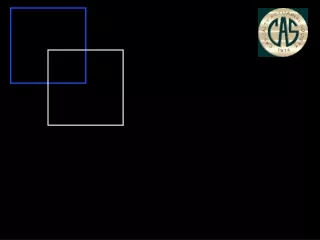
29. Greatest Accuracy CredibilityIllustration Steve Philbrick’s target shooting example... B A S1 S2 E D C

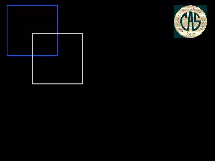
30. Greatest Accuracy CredibilityIllustration (continued) Which data exhibits more credibility? A B S1 E S2 C D

31. Greatest Accuracy CredibilityIllustration (continued) Higher credibility: less variance within, more variance between Class loss costs per exposure...  0 D A B E C Lower credibility: more variance within, less variance between D A B E C 0 

32. Greatest Accuracy CredibilityIncreasing credibility • Per the formula, Z = n n + s2 t2 • Credibility, Z, can be increased by: • Increasing n = get more data • decreasing s2 = less variance within classes, e.g., refine data categories • increase t2 = more variance between classes

33. Greatest Accuracy CredibilityStrengths and weaknesses • The greatest accuracy or least squares credibility result is more intuitively appealing. • It is a relative concept • It is based on relative variances or volatility of the data • There is no such thing as full credibility • Issues • Greatest accuracy credibility is can be more difficult to apply. Practitioner needs to be able to identify variances. • Credibility, z, is a property of the entire set of data. So, for example, if a data set has a small, volatile class and a large, stable class, the credibility of the two classes would be the same.

34. Bibliography

35. Bibliography • Herzog, Thomas. Introduction to Credibility Theory. • Longley-Cook, L.H. “An Introduction to Credibility Theory,” PCAS, 1962 • Mayerson, Jones, and Bowers. “On the Credibility of the Pure Premium,” PCAS, LV • Philbrick, Steve. “An Examination of Credibility Concepts,” PCAS, 1981 • Venter, Gary and Charles Hewitt. “Chapter 7: Credibility,” Foundations of Casualty Actuarial Science. • ___________. “Credibility Theory for Dummies,” CAS Forum, Winter 2003, p. 621

36. Introduction to Credibility