Download
1 / 116
1.16k likes | 1.24k Views
Partitioning Graphs of Supply and Demand Generalization of Knapsack Problem. Takao Nishizeki. Tohoku University. Graph. Supply Vertices and Demand Vertices. Supply Vertices. Demand Vertices. 25. 12. 4. 4. 8. 6. 5. 3. 5. 15. 13. 7. 6. 2. 10. Supply Vertices.

E N D
Partitioning Graphsof Supply and DemandGeneralization of Knapsack Problem Takao Nishizeki Tohoku University
Graph Supply Vertices and Demand Vertices Supply Vertices Demand Vertices
25 12 4 4 8 6 5 3 5 15 13 7 6 2 10 Supply Vertices Demand Vertices Graph Each Supply Vertex has a number, called Supply. Each Demand Vertex has a number,called Demand Supply Demand
4 4 4 8 8 6 6 5 5 3 5 7 6 2 10 Desired Partition partition G into connected components so that 25 12 15 13
4 4 8 6 5 3 5 7 6 2 10 25 12 15 13 Desired Partition partition G into connected components so that
4 4 8 6 5 3 5 7 6 2 10 Sum:12 Sum:23 4 4 8 6 5 3 5 Sum:12 Sum:13 7 6 2 10 Desired Partition partition G into connected components so that • each component has exactly one supply vertex, • supply is no less than the sum of demands in the component. Desired partition 25 12 15 13
4 4 8 6 5 3 5 7 6 2 10 20 10 15 13 Maximum Partition Problem (Max PP) No desired partition
4 4 A partition of a graph must satisfy (a) each component has exactly one supply vertex, (b) supply is no less than the sum of demands in the component. 8 6 5 3 5 7 6 2 10 4 4 8 6 5 3 5 7 6 2 10 Maximum Partition Problem (Max PP) (a) each component has at most one supply vertex, (b) supply is no less than the sum of demands in the component. no supply vertex 20 10 15 13
4 4 8 6 5 3 5 7 6 2 10 Sum:17 Sum: 5 4 4 8 6 5 3 5 Sum:12 Sum:7 7 6 2 10 Maximum Partition Problem (Max PP) finds a partition that maximizes the “fulfillment.” A partition of a graph must satisfy sum of demands in all components with supply vertices (a) each component has at most one supply vertex, (b) supply is no less than the sum of demands in the component if there is a supply vertex. (a) each component has at most one supply vertex, (b) supply is no less than the sum of demands in the component. 20 10 15 13
4 4 8 6 5 3 5 7 6 2 10 Sum:17 Sum: 5 4 4 8 6 5 3 5 Sum:12 Sum:7 7 6 2 10 Maximum Partition Problem (Max PP) finds a partition that maximizes the “fulfillment.” The fulfillment of this partition 17 + 5 + 12 + 7 = 41 20 10 15 13
4 4 8 6 5 3 5 7 6 2 10 Sum:19 Sum: 8 4 4 8 6 5 3 5 Sum:12 Sum:15 7 2 10 Maximum Partition Problem (Max PP) finds a partition that maximizes the “fulfillment.” The fulfillment of this partition 19 + 8 + 12 + 15 = 54 Maximum fulfillment 20 10 15 6 13
max subset sum problem (simple ver. of Knapsack) 25 4 3 6 b = 13 2 3 9 4 7 5 15 3 4 5 7 11 given set A Complexity Status Trees NP-hard Maximum Subset Sum Problem(NP-hard) instance: a set A of integers and an integer b find: a subsetC ⊆ A which maximizes the sum of integers in C s.t. the sum does not exceed b.
25 4 3 6 2 3 9 4 7 5 15 Complexity Status max subset sum problem (simple ver. of Knapsack) Trees b = 13 C NP-hard 3 4 5 7 11 given set A Maximum Subset Sum Problem(NP-hard) instance: a set A of integers and an integer b find: a subsetC ⊆ A which maximizes the sum of integers in C s.t. the sum does not exceed b.
13 3 4 5 7 11 Related Result max subset sum problem (NP-hard) Fully Polynomial-Time Approximation Scheme (FPTAS) [Ibarra and Kim ’75] Max PPfor Stars with one supply at center FPTAS: for any e, 0 < e < 1, the algorithm finds an approximation solution such that APPRO > (1–e ) OPT in time polynomial in both n and 1/e.
4 4 13 8 6 5 3 5 3 4 5 7 11 7 6 2 10 25 12 7 4 3 6 good approximation for larger classes 2 3 9 4 15 5 25 ? 15 13 Related Result max subset sum problem (NP-hard) Fully Polynomial-Time Approximation Scheme (FPTAS) [Ibarra and Kim ’75] Max PPfor Stars with one supply at center
4 4 8 6 5 3 5 7 6 2 10 25 12 15 13 Our Results (approximabiliy) General graphs (1) MAXSNP-hard (APX-hard) No PTAS unless P=NP No FPTAS unless P=NP PTAS: for any e, 0 < e < 1, the algorithm finds an approximation solution such that APPRO > (1–e ) OPT in time polynomial in n. (1/e :regarded as a constant.)
4 4 25 4 3 6 8 6 5 3 5 2 3 9 4 7 5 15 7 6 2 10 25 12 15 13 Our Results (approximabiliy) General graphs (1) MAXSNP-hard (APX-hard) No PTAS unless P=NP Trees NP-hard (2) FPTAS
4 4 25 4 3 6 8 6 5 3 5 2 3 9 4 7 5 15 7 6 2 10 25 12 15 13 Our Results (approximabiliy) General graphs (1) MAXSNP-hard (APX-hard) No PTAS unless P=NP Trees NP-hard (2) FPTAS
7 L-reduction 7 7 3-occurrence MAX3SAT Max PP for bipartite graphs 4 4 4 4 4 4 each variable appears at most 3 times 1 1 1 (1) MAXSNP-hardness Max PP is MAXSNP-hard for bipartite graphs. L-reduction: preserves approximability error ratio: e’ error ratio: e
(1) MAXSNP-hardness 3-occurrence MAX3SAT (MAXSNP-hard) • instance: variables and clauses s.t. • each clause has exactly 3 literals; and • each variable appears at most 3 times in the clauses • find: a truth assignment which maximizes # of satisfied clauses variables: v wx y z at most 3 times
at most 3 times (1) MAXSNP-hardness 3-occurrence MAX3SAT (MAXSNP-hard) • instance: variables and clauses s.t. • each clause has exactly 3 literals; and • each variable appears at most 3 times in the clauses • find: a truth assignment which maximizes # of satisfied clauses variables: v wx y z
(1) MAXSNP-hardness 3-occurrence MAX3SAT (MAXSNP-hard) • instance: variables and clauses s.t. • each clause has exactly 3 literals; and • each variable appears at most 3 times in the clauses • find: a truth assignment which maximizes # of satisfied clauses variables: v wx y z
x = true 7 7 x 4 4 4 4 x = false x x x 7 4+4 = 8> 7 x 4 4 (1) MAXSNP-hardness variable gadget variable x x
x y z x y z 7 7 7 4 4 4 4 4 4 (1) MAXSNP-hardness variable x variable y variable z 1 1 1
x y z x y z 7 7 7 4 4 4 4 4 4 (1) MAXSNP-hardness variable x variable y variable z 1 1 1
x y z x y z 7 7 7 4 4 4 4 4 4 (1) MAXSNP-hardness variable x variable y variable z 1 1 1
7 7 7 4 4 4 4 4 4 7 – 4 =3 enough power (1) MAXSNP-hardness variable x variable y variable z x y z x y z at most 3 1 1 1
7 7 7 4 4 4 4 4 4 (1) MAXSNP-hardness variable x variable y variable z x y z x y z 1 1 1
(1) MAXSNP-hardness x = true y = false z = false 7 7 7 x y z x y z 4 4 4 4 4 4 1 1 1
7 7 7 4 4 4 4 4 4 (1) MAXSNP-hardness variable x variable y variable z x y z x y z 1 1 1
(1) MAXSNP-hardness x = false y = false z = false 7 7 7 x y z x y z 4 4 4 4 4 4 not satisfied 1 1 1
7 7 7 4 4 4 4 4 4 1 1 1 (1) MAXSNP-hardness Max PP is MAXSNP-hard for bipartite graphs. L-reduction: preserves approximability L-reduction 3-occurrence MAX3SAT Max PP for bipartite graphs each variable appears at most 3 times
4 4 25 4 3 6 8 6 5 3 5 2 3 9 4 7 5 15 7 6 2 10 25 12 15 13 Our Results (approximabiliy) General graphs (1) MAXSNP-hard (APX-hard) No PTAS unless P=NP Trees NP-hard (2) FPTAS Pseudo-poly.-time algorithm
25 4 3 6 2 3 9 4 7 • sum of all demands • sum of all supplies 5 15 F = min 2+3+4+・・・+4+5= 43 15+25= 40 Pseudo-Polynomial-Time Algorithm Max PP is NP-hard even for trees. Max PP can be solved for a tree T in time O(F2n) if the supplies and demands are integers. F= min{43,40}=40 max fulfillment ≦ F
root 3 4 7 7 2 8 2 4 3 6 5 2 3 9 4 20 20 5 15 25 Pseudo-Polynomial-Time Algorithm Dynamic Programming 20 2 7 2 4 25 4 3 6 9 root 8 2 7 5 15 5 3 4 3 20
5 5 5 Tv 10 Tv v 9 10 10 9 9 20 5 3 20 20 5 5 3 3 Pseudo-Polynomial-Time Algorithm T optimal partition of Tv optimal partition of T 5 v 10 9 20 5 3 fulfillment=18 fulfillment=20
marginal power 20-(10+5+3)=2 5 5 5 10 20-10= Tv Tv v 10 10 10 9 9 9 20 5 3 20 20 5 5 3 3 fulfillment: 10 Pseudo-Polynomial-Time Algorithm Dynamic Programming 5 v 10 9 20 5 3 fulfillment: 18
20-(10+3)= 7 20-(10+5)=5 5 5 5 Tv Tv v 10 10 9 9 9 20 20 5 5 3 3 fulfillment: 15 Pseudo-Polynomial-Time Algorithm Dynamic Programming 5 v 10 10 9 20 20 5 5 3 3 fulfillment: 13
optimal partition of T 10 2 5 5 Tv Tv v v 10 10 9 10 10 9 5 5 5 5 5 5 20 20 5 5 3 3 20 20 5 5 3 3 Tv v 9 9 9 9 10 10 9 9 fulfillment: 18 fulfillment: 10 5 5 7 5 Tv Tv 20 20 5 5 3 3 v v 10 10 9 10 10 9 20 20 5 5 3 3 20 20 5 5 3 3 fulfillment: 13 fulfillment: 15 Pseudo-Polynomial-Time Algorithm
marginal power 10 2 5 5 Tv Tv v v 10 10 9 10 10 9 5 5 5 5 20 20 5 5 3 3 20 20 5 5 3 3 9 9 9 9 fulfillment: 18 fulfillment: 10 3 2 5 5 7 5 1 F Tv Tv v v 10 10 9 10 10 9 0 1 2 3 fulfillment 20 20 5 5 3 3 20 20 5 5 3 3 F points fulfillment: 13 fulfillment: 15 Pseudo-Polynomial-Time Algorithm staircase,non-increasing
deficient power 5+4=9 5 5 Tv Tv v v 5 5 15 15 3 3 4 4 5 5 Pseudo-Polynomial-Time Algorithm optimal partition of T 5 Tv v 5 15 3 4 5 fulfillment: 9
optimal partition of T 5 8 5 5 Tv Tv 5 15 5 15 5 5 v v 3 4 5 3 4 5 Tv Tv v v 5 5 15 15 fulfillment: 8 fulfillment: 5 9 12 5 5 3 3 4 4 5 5 Tv Tv 5 15 5 15 v v 3 4 5 3 4 5 fulfillment: 12 fulfillment: 9 Pseudo-Polynomial-Time Algorithm
deficient power 5 8 5 5 Tv Tv 5 15 5 15 v v 3 4 5 3 4 5 fulfillment: 8 fulfillment: 5 3 2 9 12 5 5 1 F Tv Tv 5 15 5 15 v v 0 1 2 3 fulfillment 3 4 5 3 4 5 F points fulfillment: 12 fulfillment: 9 Pseudo-Polynomial-Time Algorithm staircase, non-decreasing
3 4 7 7 2 8 2 4 3 6 5 2 3 9 4 20 20 5 15 25 Pseudo-Polynomial-Time Algorithm leaves
marginal power deficient power F F 3 fulfillment 0 fulfillment 2 0 3 1 1 2 3 4 7 7 2 8 2 4 3 6 3 O(F2) time 5 2 3 9 4 20 20 4 7 7 5 15 25 deficient power marginal power deficient power 2 8 2 4 3 6 marginal power F 5 2 3 9 4 20 20 F F F 0 2 3 1 fulfillment 0 2 3 1 0 1 2 3 fulfillment fulfillment 5 15 25 fulfillment 0 1 2 3 Pseudo-Polynomial-Time Algorithm
deficient power marginal power F F root 0 3 0 2 fulfillment 3 1 1 2 3 fulfillment 4 7 7 Dynamic Programming 2 8 2 4 3 6 5 2 3 9 4 20 20 5 15 25 Pseudo-Polynomial-Time Algorithm max fulfillment
root 3 4 7 7 Dynamic Programming 2 8 2 4 3 6 5 2 3 9 4 20 20 5 15 25 Pseudo-Polynomial-Time Algorithm Computation time for each vertex ・・・・・・・・・・・・・・O(F2) There are n vertices.
Computation time for each vertex ・・・・・・・・・・・・・・O(F2) Pseudo-Polynomial-Time Algorithm There are n vertices. Computation time O(F2n) The algorithm takes polynomial timeif F is bounded by a polynomial in n.
(2) FPTAS Let all demands and supply be positive real numbers. For any e, 0< e <1, the algorithm finds a partition of a tree T such that OPT – APPRO < e OPT in time polynomial in both n and 1/e . n : # of vertices
marginal power 0 t fulfillment (2) FPTAS The algorithm is similar to the previous algorithm. sampled fulfillment