QUANTITATIVE ANALYSIS
QUANTITATIVE ANALYSIS. MBA BOOK REVIEW MICASA HOTEL 19th October 2002. Zuwailiah Jamaludin October 2002. QUANTITATIVE ANALYSIS. DECISION TREE ANALYSIS. CASH FLOW ANALYSIS. NET PRESENT VALUE. PROBABILITY THEORY. REGRESSION ANALYSIS & FORECASTING. DECISION TREE ANALYSIS. Objective :.

QUANTITATIVE ANALYSIS
E N D
Presentation Transcript
QUANTITATIVE ANALYSIS MBA BOOK REVIEW MICASA HOTEL 19th October 2002 Zuwailiah Jamaludin October 2002
QUANTITATIVE ANALYSIS DECISION TREE ANALYSIS CASH FLOW ANALYSIS NET PRESENT VALUE PROBABILITY THEORY REGRESSION ANALYSIS & FORECASTING
DECISION TREE ANALYSIS Objective : Break complex problems into manageable parts How? DECISION TREE DIAGRAM 5 steps > • Determine all possible alternatives and risks • Calculate monetary consequence of alternatives • Determine uncertainty of each alternatives • Combine top three steps into a tree diagram • Determine the best alternative & • consider non- monetary aspects
For different alternatives EVENT FORKS ACTIVITY FORKS
To drill or not to drill 1. Paid $20,000 for drill option 2.Could lower risk if hire a geologist to perform seismic testing at $50,000. T gives better indication of success and lower risks. 3. Should he proceed with drilling option at $ 200,000 4. Consulted oil experts says the land has 60% chance of having oil 5. If seismic tests show positive for oil, it has a 90% chance of having oil 6. If seismic tests show negative for oil, it has a 10% chance of having oil
2. Build the tree 0.9 oil DRILL dry 0.1 0.60 +ve 0.1 oil NO DRILL DRILL -ve TEST dry 0.40 0.9 NO DRILL 0.6 oil NO TEST DRILL dry 0.4 NO DRILL
3. Calculate Expected Monetary Value (EMV) (Expected income $ 1 Million) 0.9 (1,000,000 x 0.9) + (0 x 0.1) = $ 900,000 0.1 0.60 0.1 (1,000,000 x 0.1) + (0 x 0.9) = $ 100,000 0.40 0.9 0.6 (1,000,000 x 0.6) + (0 x 0.4) = $ 600,000 0.4 > use of activity squares to choose the best outcome
4. to determine best alternative, subtract applicable cost 0.9 EMV > cost Drill $900K $700K Drill -$200K 0.1 0.60 $420K EMV < cost No drill 0.1 Test -$50K $100K -$200K 0.40 0.9 EMV > cost Drill 0.6 $600K $400K -$200K 0.4
Recap : Work from Right to Left of the tree 1. Multiply outcome of probabilities = EMV of drill 2. Choose to drill if EMV > cost 3. Choose to test or not by choosing the highest EMV
CASH FLOW ANALYSIS > basis of financial analysis Goal : Determine WHEN and HOW MUCH cash flow in a given scenario Answers the question …. What does the investment cost (current investment) and how much will it generate (future benefits) each year
Answers the question …. What does the investment cost (current investment) and how much will it generate (future benefits) each year Steps taken to answer the questions ….. 1. Define the VALUE of the investment 2. Calculate the MAGNITUDE of the benefits 3. Determine the TIMING of the benefits 4. Quantify the UNCERTAINTY of the benefits 5. Do the benefits JUSTIFY the wait?
To determine the cash uses during the life of project • CASH SOURCES • Revenue or sales • Royalties • CASH USES • COGS • Selling cost • General & Admin cost • Taxes
> Does not indicate PROFIT Profits (from acct statement) short-term measurement of investment in a shorter time-frame than the life of the investment Cash Flow analysis is a technique used to evaluate individual projects over the life of the project. VS > Depreciation is not relevant > Financing costs are not included
Eg of cash flow : refer to notes …. > Indicate how timing is important ….. A +$61 +$51 +$51 -$102 Year 1 Year 2 Year 3 Year 4 +$163 B -$102
ACCUMULATED VALUE Assumption : In company can reinvest with a 10% yield B Future value of a $ in x periods = ($today) x (1+Reinvestment rate) No of period > $1 x (1+.10)¹ = 1.10 Use basic business calculator to get the accumulated value $1 today = $1 today $1 invested = $ 1.1 in 1 yr $1 invested = $ 1.21 in 2 yrs In this case >>>>> $ 34230
CONCLUSION In evaluating projects / investments that extend into future, one must consider , 1. MAGNITUDE OF CASH FLOW 2. TIMING OF CASH 3. SUBSEQUENT USE OF CASH • Cash flow analysis determines the flow but we need to value • the cash in today’s dollars. • Only then can we compare different projects regardless of • timing
NET PRESENT VALUE (NPV) NPV analysis takes future cash flows and discounts them to their present -day value > Note : This is the inverse of accumulated value > $1 x (1+.10)-¹ = 0.90909 Discount factor Future Cash x Discount Factor = NPV
Future Cash x Discount Factor = NPV Yr 0 $ 102,000 x 1 = - $ 102,000.00 Yr 1 $ 51,000 x 0.90909 = $ 46,363.59 Yr 2 $ 51,000 x 0.82645 = $ 42,148.95 Yr 3 $ 61,000 x 0.75131 = $ 45829.91 NPV$ 32,342.40 In evaluating projects / investments that extend into future, one must consider , 1. MAGNITUDE OF CASH FLOW 2. TIMING OF CASH 3. SUBSEQUENT USE OF CASH 4. DISCOUNT RATE
Discount Rate = Hurdle rate Discount Rate Hurdle rate What determines the Discount Rate ? • Subjective • Depends on the risks • Under no circumstances that the bank’s debt rate be used
INTERNAL RATE OF RETURN (IRR) The rate at which the discounted cash flows in the future equal the value of investment today ie discounted rate used to get NPV = 0 HOW? 1. Try different discount rate until NPV =0 2. Use HP calculator Use discount factor : 26.709% Yr 0 $ 102,000 x 1 = - $ 102,000.00 Yr 1 $ 51,000 x 0.78920 = $ 40250.00 Yr 2 $ 51,000 x 0.62285 = $ 31,765.00 Yr 3 $ 61,000 x 0.49155 = $ 29985.00 NPV$ 0
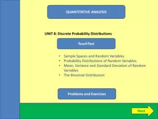
PROBABILITY THEORY Probability Distributions • Multiple outcomes result in a distribution of outcomes • Each possibility is assigned a probability • Graph showing distribution of outcomes is called a • probability mass / density function Normal Distribution = Bell Curve When a probability mass function is based on many trials, the curve tends to become bell-shaped
P % This hump is caused by CENTRAL LIMIT THEOREM states that “distribution of averages of repeated independent samples will take the form of the bell-shaped normal distribution” MEASURES OF NORMAL CURVE : MEAN = centre of curve / average STD DEVIATION (SD) = how wide the curve appears MEDIAN = centre MODE = highest value
CUMULATIVE DISTRIBUTION FUNCTION (CDF) - a cumulative view of a probability function Normal curve tells you probability of a given outcome but CDF tells you probability of a range of values. P $
REGRESSION ANALYSIS & FORECASTING Linear regression models are used to determine relationships between variables that are related Once a relationship is established, the future can be forecast • Regression analysis involves gathering data to determine • relationships of variables • Goal of regression is to produce an equation of a line that • depicts the relationship
Y * Y=mX + b sales * Y = dependant variable m = slope of line ( relationship) X = independent variable b = y axis intercept * * * * m * b X temp 35 Eg : To know sales at 35 degrees b= 15000 m= 5 Y = (5 x 35) + 15000 = 32500 At 35 degrees temp, sale is expected at RM 32500
SUMMARY • Sort out complex problems with decision trees • Determine the cash received in the future - cash flow • analysis and net present value analysis • Quantify uncertainty with probability theory • Determine relationships and forecast with regression • analysis