Download
1 / 26
270 likes | 533 Views
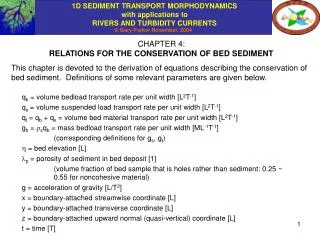
CHAPTER 4: RELATIONS FOR THE CONSERVATION OF BED SEDIMENT. This chapter is devoted to the derivation of equations describing the conservation of bed sediment. Definitions of some relevant parameters are given below. . q b = volume bedload transport rate per unit width [L 2 T -1 ]

E N D
CHAPTER 4: RELATIONS FOR THE CONSERVATION OF BED SEDIMENT This chapter is devoted to the derivation of equations describing the conservation of bed sediment. Definitions of some relevant parameters are given below. • qb = volume bedload transport rate per unit width [L2T-1] • qs = volume suspended load transport rate per unit width [L2T-1] • qt = qb + qs = volume bed material transport rate per unit width [L2T-1] • gb = sqb = mass bedload transport rate per unit width [ML-1T-1] • (corresponding definitions for gs, gt) • = bed elevation [L] p = porosity of sediment in bed deposit [1] (volume fraction of bed sample that is holes rather than sediment: 0.25 ~ 0.55 for noncohesive material) g = acceleration of gravity [L/T2] x = boundary-attached streamwise coordinate [L] y = boundary-attached transverse coordinate [L] z = boundary-attached upward normal (quasi-vertical) coordinate [L] t = time [T]
COORDINATE SYSTEM x = nearly horizontal boundary-attached “streamwise” coordinate [L] y = nearly horizontal boundary-attached “transverse” coordinate [L] z = nearly vertical coordinate upward normal from boundary [L]
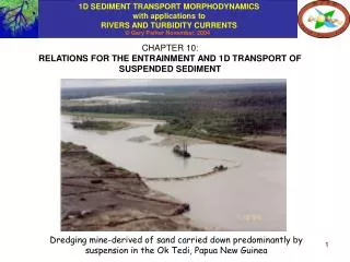
ILLUSTRATION OF BEDLOAD TRANSPORT Double-click on the image to see a video clip of bedload transport of 7 mm gravel in a flume (model river) at St. Anthony Falls Laboratory, University of Minnesota. (Wait a bit for the channel to fill with water.) Video clip from the experiments of Miguel Wong. rte-bookbedload.mpg: to run without relinking, download to same folder as PowerPoint presentations.
CASE OF 1D, BEDLOAD ONLY, SEDIMENT APPROXIMATED AS UNIFORM IN SIZE or thus This corresponds to the original form derived by Exner.
2D GENERALIZATION, BEDLOAD ONLY (Yes, this is still a course on 1D morphodynamics, but it is useful to know the 2D form.) where denote unit vectors in the x and y directions.
ILLUSTRATION OF MIXED TRANSPORT OF SUSPENDED LOAD AND BEDLOAD Double-click on the image to see the transport of sand and pea gravel by a turbidity current (sediment underflow driven by suspended sediment) in a tank at St. Anthony Falls Laboratory. Suspended load is dominant, but bedload transport can also be seen. Video clip from experiments of Alessandro Cantelli and Bin Yu. rte-bookturbcurr.mpg: to run without relinking, download to same folder as PowerPoint presentations.
CASE OF 1D BEDLOAD + SUSPENDED LOAD Es = volume rate per unit time per unit bed area that sediment is entrained from the bed into suspension [LT-1]. Ds = volume rate per unit time per unit bed area that sediment is deposited from the water column onto the bed [LT-1]. or thus
EVALUATION OF Ds AND Es Let denote the volume concentration of sediment c in suspension at (x, z, t), averaged over turbulence. Here c = (sediment volume)/(water volume + sediment volume). In the case of a dilute suspension of non-cohesive material, where cb denotes the near-bed value of c . Similarly, a dimensionless entrainment rate E can be defined such that Thus
CASE OF 1D BEDLOAD + SUSPENDED LOAD, ADDITION OF TECTONICS (SUBSIDENCE OR UPLIFT) The analysis below is based on Paola et al. (1992). Conserve bed sediment between some base level z = base(x, t) and the bed surface : The tectonic subsidence rate (uplift rate ) is given as Thus with the previously-presented evaluations for Es and Ds: 2D generalization:
TRANSPORT RATE OF SUSPENDED SEDIMENT Definitions: z = upward normal coordinate from the bed [L] = local streamwise flow velocity averaged over turbulence [L/T] = local volume sediment concentration averaged over turbulence [1] H = flow depth [L] qs = volume transport rate of suspended sediment per unit width [L2/T] U = vertically averaged streamwise flow velocity [L/T] C = vertically flux-averaged volume concentration of sediment in suspension [1] z
1D EQUATION OF CONSERVATION OF SEDIMENT IN SUSPENSION (mass of sediment in control volume)/t = net mass inflow rate of suspended sediment + mass rate of entrainment of sediment into suspension – mass rate of deposition onto the bed or reducing with the relation qs = UCH and previous evaluations for Es and Ds,
REDUCTION: 1D EXNER FORMULATION IN TERMS OF TOTAL BED MATERIAL LOAD In most cases the condition << 1 prevails, allowing the approximation The simplified form of the above equation can be combined with the Exner equation of conservation of bed sediment, to yield the following form for Exner: or defining total bed material load qt = qb + qs,
2D GENERALIZATION, TOTAL BED MATERIAL LOAD Let denote the local average velocity in the transverse (y) direction. Then Now Thus
1D CONSERVATION OF BED SEDIMENT FOR SIZE MIXTURES, BEDLOAD ONLY fi'(z', x, t) = fractions at elevation z' in ith grain size range above datum in bed [1]. Note that over all N grain size ranges: qbi(x, t) = volume bedload transport rate of sediment in the ith grain size range [L2/T] Or thus:
ACTIVE LAYER CONCEPT The active, exchange or surface layer approximation (Hirano, 1972): Sediment grains in active layer extending from - La < z’ < have a constant, finite probability per unit time of being entrained into bedload. Sediment grains below the active layer have zero probability of entrainment.
REDUCTION OF SEDIMENT CONSERVATION RELATION USING THE ACTIVE LAYER CONCEPT Fractions Fi in the active layer have no vertical structure. Fractions fi in the substrate do not vary in time. Thus where the interfacial exchange fractions fIi defined as describe how sediment is exchanged between the active, or surface layer and the substrate as the bed aggrades or degrades.
REDUCTION OF SEDIMENT CONSERVATION RELATION USING THE ACTIVE LAYER CONCEPT contd. Between and it is found that (Parker, 1991).
REDUCTION contd. The total bedload transport rate summed over all grain sizes qbT and the fraction pbi of bedload in the ith grain size range can be defined as The conservation relation can thus also be written as Summing over all grain sizes, the following equation describing the evolution of bed elevation is obtained: Between the above two relations, the following equation describing the evolution of the grain size distribution of the active layer is obtained:
EXCHANGE FRACTIONS where 0 1 (Hoey and Ferguson, 1994; Toro-Escobar et al., 1996). In the above relations Fi, pbi and fi denote fractions in the surface layer, bedload and substrate, respectively. That is: The substrate is mined as the bed degrades. A mixture of surface and bedload material is transferred to the substrate as the bed aggrades, making stratigraphy. Stratigraphy (vertical variation of the grain size distribution of the substrate) needs to be stored in memory as bed aggrades in order to compute subsequent degradation.
1D GENERALIZATIONS: TECTONICS, SUSPENSION, TOTAL BED MATERIAL LOAD To include tectonics, make the transformation - base in the above derivation (or integrate from z’’ = 0 to z’’ = - base, where z’’ = z’ - base) to obtain: To include suspended sediment, let vsi = fall velocity, Ei = dimensionless entrainment rate, and denote the near-bed volume concentration of sediment, all for the ith grain size range, so that the relation generalizes to: Repeating steps outlined previously for uniform sediment, if qtT denotes the total bed material load summed over all sizes and pti denotes the fraction of the bed material load in the ith grain size range,
WHY THE CONCERN WITH SEDIMENT MIXTURES? Rivers often sort their sediment. An example is downstream fining: many rivers show a tendency for sediment to become finer in the downstream direction. bed slope elevation Long profiles showing downstream fining and gravel-sand transition in the Kinu River, Japan (Yatsu, 1955) median bed material grain size
upstream downstream WHY THE CONCERN WITH SEDIMENT MIXTURES ? contd. Downstream fining can also be studied in the laboratory by forcing aggradation of heterogeneous sediment in a flume. Downstream fining of a gravel-sand mixture at St. Anthony Falls Laboratory, University of Minnesota (Toro-Escobar et al., 2000) Many other examples of sediment sorting also motivate the study of the transport, erosion and deposition of sediment mixtures.
FURTHER PROGRESS Sediment approximated as uniform in size Sediment mixtures • In order to make further progress, it is necessary to • Develop a means for computing the bedload transport rate qb (qbi) as a function of the flow; • Develop a means for computing the dimensionless entrainment rate E (Ei) into suspension as a function of the flow; • Develop a model for tracking the concentration of sediment in suspension, so that can be computed. • Specify the thickness of the active layer La. • The key flow parameter turns out to be boundary shear stress .
REFERENCES FOR CHAPTER 4 Hirano, M., 1971, On riverbed variation with armoring, Proceedings, Japan Society of Civil Engineering, 195: 55-65 (in Japanese). Hoey, T. B., and R. I. Ferguson, 1994, Numerical simulation of downstream fining by selective transport in gravel bed rivers: Model development and illustration, Water Resources Research, 30, 2251-2260. Paola, C., P. L. Heller and C. L. Angevine, 1992, The large-scale dynamics of grain-size variation in alluvial basins. I: Theory, Basin Research, 4, 73-90. Parker, G., 1991, Selective sorting and abrasion of river gravel. I: Theory, Journal of Hydraulic Engineering, 117(2): 131-149. Toro-Escobar, C. M., G. Parker and C. Paola, 1996, Transfer function for the deposition of poorly sorted gravel in response to streambed aggradation, Journal of Hydraulic Research, 34(1): 35-53. Toro-Escobar, C. M., C. Paola, G. Parker, P. R. Wilcock, and J. B. Southard, 2000, Experiments on downstream fining of gravel. II: Wide and sandy runs, Journal of Hydraulic Engineering, 126(3): 198-208. Yatsu, E., 1955, On the longitudinal profile of the graded river, Transactions, American Geophysical Union, 36: 655-663.