Some 2-D Data (X)
3 “Products” of Principle Component Analysis. Singular Value Decomposition (SVD) X = U S V T. 1) Eigenvectors. Some 2-D Data (X). 2) Eigenvalues. 3) Principle Components. Eigenanalysis XX T = C; CE = L E. Examples for Today. 1) Eigenvectors – Variations explained in the horizontal.

Some 2-D Data (X)
E N D
Presentation Transcript
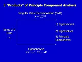
3 “Products” of Principle Component Analysis Singular Value Decomposition (SVD)X = USVT 1) Eigenvectors Some 2-D Data (X) 2) Eigenvalues 3) Principle Components Eigenanalysis XXT = C; CE = LE
Examples for Today 1) Eigenvectors – Variations explained in the horizontal Photo (X) 2) Eigenvalues - % of Variance explained 3) Principle Components Variations explained in the vertical 1) Eigenvectors – Variations explained in space (MAPS) Fake and Real Space-Time Data (X) 2) Eigenvalues - % of Variance explained (spectrum) 3) Principle Components Variations explained in the time (TIMESERIES)
Examples for Today 1) Eigenvectors – Variations explained in space (MAPS) Fake and Real Space-Time Data (X) 2) Eigenvalues - % of Variance explained (spectrum) 3) Principle Components Variations explained in the time (TIMESERIES)
Eigenvectors, Eigenvalues, PC’s • Eigenvectors explain variance in one dimension; Principle components explain variance in the other dimension. • Each eigenvector has a corresponding principle component. The PAIR define a mode that explains variance. • Each eigenvector/PC pair has an associated eigenvalue which relates to how much of the total variance is explained by that mode.
EOF’s and PC’s for geophysical data • For geophys. data, we often set it up so that the eigenvectors give us spatial structures (EOFs – empirical orthogonal functions) and the PC’s give us an associated time series (principle components) . • The EOF’s and PC’s are constructed to efficiently explain the maximum amount of variance in the data set. • In general, the majority of the variance in a data set can be explained with just a few EOFs.
EOF’s and PC’s for geophysical data • By construction, the EOFs are orthogonal to each other, as are the PCs. • Provide an ‘objective method’ for finding structure in a data set, but interpretation requires physical facts or intuition.
Variance of Northern Hemisphere Sea Level Pressure Field in Winter
PCA for the REAL Sea-Level Pressure Field EOF 1: AO/NAM (23% expl). EOF 2: PNA (13% expl.) EOF 3: non-distinct(10% expl.)
EOF 1 (AO/NAM) EOF 2 (PNA) EOF 3 (?) PC 1 (AO/NAM) PC 2 (PNA) PC 3 (?)
EOF 1 EOF 2 PC 1 PC 2
EOF 1 - 60% variance expl. EOF 2 - 40% variance expl. PC 1 PC 2
Eigenvalue Spectrum EOF 1 - 60% variance expl. EOF 2 - 40% variance expl. PC 1 PC 2
EOF 1 - 65% variance expl. EOF 2 - 35% variance expl. PC 1 PC 2
Significance First 25 Eigenvalues for DJF SLP • Each EOF / PC pair comes with an associated eigenvalue • The normalized eigenvalues (each eigenvalue divided by the sum of all of the eigenvalues) tells you the percent of variance explained by that EOF / PC pair. • Eigenvalues need to be well separated from each other to be considered distinct modes.
These two just barely overlap. Need physical intuition to help judge. Example of overlapping eigenvalues Significance: The North Test First 25 Eigenvalues for DJF SLP • North et al (1982) provide estimate of error in estimating eigenvalues • Requires estimating DOF of the data set. • If eigenvalues overlap, those EOFs cannot be considered distinct. Any linear combination of overlapping EOFs is an equally viable structure.
Validity of PCA modes: Questions to ask • Is the variance explained more than expected for null hypothesis (red noise, white noise, etc.)? • Do we have an a priori reason for expecting this structure? Does it fit with a physical theory? • Are the EOF’s sensitive to choice of spatial domain? • Are the EOF’s sensitive to choice of sample? If data set is subdivided (in time), do you still get the same EOF’s?
Regression Maps vs. Correlation Maps PNA - Regression map (meters/std deviation of index) PNA - Correlation map (r values of each point with index)
Practical Considerations • EOFs are easy to calculate, difficult to interpret. There are no hard and fast rules, physical intuition is a must. • Due to the constraint of orthogonality, EOFs tend to create wave-like structures, even in data sets of pure noise. So pretty… so suggestive… so meaningless. Beware of this.
Practical Considerations • EOF’s are created using linear methods, so they only capture linear relationships. • By nature, EOF’s give are fixed spatial patterns which only vary in strength and in sign. E.g., the ‘positive’ phase of an EOF looks exactly like the negative phase, just with its sign changed. Many phenomena in the climate system don’t exhibit this kind of symmetry, so EOF’s can’t resolve them properly.