Market Analysis & Position Sizing (Both Equally Necessary)
700 likes | 900 Views
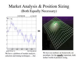
Market Analysis & Position Sizing (Both Equally Necessary). =. We have no method, no framework, no paradigm, for the equally important, dark nether-world of position sizing. We have a plethora of market analysis, selection and timing techniques…..but. Part 1. Optimal f.

Market Analysis & Position Sizing (Both Equally Necessary)
E N D
Presentation Transcript
Market Analysis & Position Sizing(Both Equally Necessary) = We have no method, no framework, no paradigm, for the equally important, dark nether-world of position sizing. We have a plethora of market analysis, selection and timing techniques…..but
Part 1 Optimal f
Everyone, on Every Trade, on Every “Opportunity” Involving Risk, has an f value (whether they acknowledge it or not): f = | Biggest Losing Outcome for 1 Unit | / f$ f$ = Account Equity / Units Where: (also f$ = | Biggest Losing Outcome for 1 Unit | / f Example: -$10,000 Biggest Losing Outcome, $50,000 Account, and I have on 200 shares, (2 units ): f$ = 50,000 / 2 = 25,000 f = | -10,000 | / 25,000 = .4
f$ and GHPR Invariant to Biggest Loss BiggestLoss ff$ GHPR –0.6 .15 4 1.125 –1 .25 4 1.125 –2 .5 4 1.125 –5 1.25 4 1.125 –29 7.25 4 1.125
The distribution can be made into bins. A scenario is a bin. It has a probability and An outcome (P/L)
Mathematical Expectation 2:1 coin toss: ME = .5 * -1 + .5 * 2 = -.5+1 = .5
f value example – 2:1 Coin Toss • $10 stake • Worst Case Outcome -1 • I’m wagering $5 (5 units) • f$ = 10 / 5 = 2 (one bet for every $2 in my stake) • f =|-1| / 2 = .5 • When biggest loss is manifest, we lose f% of our stake – 50% in this case
The Mistaken Impression Multiple made on stake = 1 + ME/|BL| * f (a.k.a Holding Period Return, “HPR”)
f after 40 plays 40 Plays 1 Play
f after 40 plays At .15 and .40, makes the same, but drawdown changes At f=.1 and .4, makes the same, But drawdown changes!
f after 40 plays Beyond .5, even in this very favorable game, TWR (multiple) < 1, meaning you are losing money and will eventually go broke if you continue
f after 40 plays Points of Inflection: Concave up to concave down. Up has gain growing faster than drawdown.(but these too migrate to the optimal point as the number of holding periods grows!)
Most Favorable Blackjack Condition Optimal f = .06 or risk $1 for every $16.67 in stake
Part 2 The Leverage Space Portfolio Model
Why The Leverage Space Model is Superior to Traditional (Modern Portfolio Theory) Models: • Risk is defined as drawdown, not variance in returns. • The fallacy and danger of correlation is eliminated. • Valid for any distributional form – fat tails are addressed. • The Leverage Space model is about leverage, which is not addressed in the traditional models.
Leverage has 2 Axes – 2 Facets The instant case of how much I am levered up f How I progress my quantity with respect to time / equity changes
The fallacy and danger of correlation • Fails when you are counting on it the most – at the (fat) tails of the distribution. • Traditional models depend on correlation – Leverage Space model does not. • cl/gc (all days) r=.18 (cl>3sd) r=.61 (cl<1sd) r=.09 • f/pfe (all days) r=.15 (sp>3sd) r=.75 (sp<1sd) r=.025 • c/msft (all days)r=.02 (gc>3sd) r=.24 (gc<1sd) r=.01
Why The Leverage Space Model is Superior to Traditional (Modern Portfolio Theory) Models: • Risk is defined as drawdown, not variance in returns. • The fallacy and danger of correlation is eliminated. • Valid for any distributional form – fat tails are addressed. • The Leverage Space model is about leverage, which is not addressed in the traditional models. (on both axes of “Leverage”)
Part 3 The Leverage Space Model Software Implementation
Link for how to gather your data and create scenarios & probabilities: http://parametricplanet.com/rvince/ScenariosExample.xls
Here is the data I am using (this is from the link example from the previous slide) :
Date,Equity Jan-07,617.00 Feb-07,664.00 Mar-07,673.00 Apr-07,751.00 May-07,887.00 Jun-07,849.00 Jul-07,781.00 Aug-07,851.00 Sep-07,942.00 Oct-07,834.00 Nov-07,804.00 Dec-07,789.00 Jan-08,791.00 Feb-08,813.00
Get java at: http://java.com/en/download/index.jsp