Transportation Problem
Transportation Problem. Lecture 19 By Dr. Arshad Zaheer. RECAP. T ransportation model Illustration (Demand = Supply) Optimal Solution Stepping Stone Method Modi Method. Total Capacity (Supply) exceeds Total Demand. Illustration 1. Minimize the transportation cost . Solution.

Transportation Problem
E N D
Presentation Transcript
Transportation Problem Lecture 19 By Dr. Arshad Zaheer
RECAP Transportation model Illustration (Demand = Supply) Optimal Solution Stepping Stone Method Modi Method
Illustration 1 Minimize the transportation cost
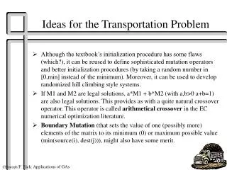
Solution In this case we will introduce the fictitious destinations with demand equal to the difference of total capacity and total demands at zero cost of transportation from sources to fictitious destinations or at the cost stated in problem. We then use transportation algorithm to find the optimal solution.
Initial Solution by Least Cost First Rule In Df column all the cells have 0 cost which is least one, we can select any one of them to be filled first. We selected S1Df cell, see its column total which is 15 and row total which is also 15. We place the less no in the box so is 15. Now the column total has been exhausted/filled and we give zero to column total in cell below. Row total also decreases to zero.
Initial Solution by Least Cost First Rule S2D3 cell has the lowest cost equal to 3 , See its column total which is 30 and row total which is 25. We place the less no in the cell so is 25. Row total has been exhausted/filled and we give zero to remaining cells while column total has been decreased to only 5
Initial Solution by Least Cost First Rule Now S3D2 cell has the lowest cost equal to 8 , See its column total which is 20 and row total which is 45. We place the less no in the cell so is 20. Column total has been exhausted/filled while row total has been decreased to only 25
Initial Solution by Least Cost First Rule Now S3D1 cell has the lowest cost equal to 12 , See its column total which is 20 and row total which is 25. we place the less no in the cell so is 20. Column total has been exhausted/filled while row total has been decreased to only 5
Initial Solution by Least Cost First Rule Last remaining cell is S3D3 which has its column total and row total equal to 5. The total is same for both sides so we place 5 in the cell
Initial Solution by Least Cost First Rule This is the initial feasible solution. Rewrite the tableau with its capacity and demand
No of Basic Variables= m+n-1 =3+4-1 =6 m= No of sources n= No of destinations
There are only five basic variables so we need another variable as a basic variables
Equations U1+V4=0 let U2=0 U2+V3=3 U1= V1=-5 U3+V1=12 U2=O V2=-9 U3+V2=8 U3=17 V3=3 U3+V3=20 V4= By using these equations when we calculate values we are unable to find the values of U1 and V4. it is due to less no of basic variables
We add epsilon which is slightly greater than 0 , this addition makes the non basic variable as basic variable this is slightly higher than zero so it does not affect the balance. We can add epsilon in any cell of column of V4 or in row of U1.
Equations Now we have another basic variable we write its equation. Addition of this new equation help us to find the values for U1 and V4 U1+V4=0 let U2=0 U2+V3=3 U1=15 V1=-5 U3+V1=12 U2=O V2=-9 U3+V2=8 U3=17 V3=3 U3+V3=20 V4=-15 U1+V1=10
Shadow cost of S1D1 Vij = (Ui + Vj) –Cij V11 = (U1 + V1) –C11 =(15-5) -10 =0 ZERO shadow cost indicates that it is a basic variable In this way we calculate the shadow cost of all the cells Shadow cost of S1D3 Vij = (Ui + Vj) –Cij V13 = (U1 + V3) –C13 =(15+3) -22 =-4
One shadow cost is positive so we use the addition and subtraction of θ
Total cost Total cost = Xij * Cij Total is calculated on the basis of all the basic variables because non basic variables are zero and their cost will also becomes zero when multiplied with zero units. = 25*3+ 20*12 + 20*8 + 5*20 =575 Max θ= Min (15,20) = 15
Equations U1+V1=10 let U2=0 U2+V3=3 U1=15 V1=-5 U3+V1=12 U2=O V2=-9 U3+V2=8 U3=17 V3=3 U3+V3=20 V4=-17 U3+V4=0
All the shadow costs are non positive so the conditions for optimality has been satisfied
If the conditions does not satisfy than we will use the previous process of addition of θ and further tabulation till the conditions satisfied, presence or absence of epsilon does not affect the solution so its up to you, whether to retain it or just drop it.
Total Cost • Total cost= 15*10 + 25*3 + 5*12 + 20*8 + 5*20 = 150 + 75 + 60 + 160 +100 = 545
Optimal Distribution S1 ─ ─ ─ ─ > D1 = 15 S2 ─ ─ ─ ─ > D3 = 25 S3 ─ ─ ─ ─ > D1 = 5 S3 ─ ─ ─ ─ > D2 = 20 S3 ─ ─ ─ ─ > D3 = 5 S3 ─ ─ ─ ─ > Df = 15 Total = 85 • Total cost= 15*10 + 25*3 + 5*12 + 20*8 + 5*20 =545