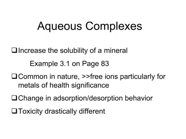
Aqueous Complexes
Aqueous Complexes. Why do we care?? Complexation of an ion also occuring in a mineral increases solubility Some elements occur as complexes more commonly than as free ions Adsorption of elements greatly determined by the complex it resides in


Aqueous Complexes
E N D
Presentation Transcript
Aqueous Complexes • Why do we care?? • Complexation of an ion also occuring in a mineral increases solubility • Some elements occur as complexes more commonly than as free ions • Adsorption of elements greatly determined by the complex it resides in • Toxicity/ bioavailability of elements depends on the complexation
Defining Complexes • Use equilibrium expressions: DG0R = -RT ln Keq • cC + lHL CL + lH+ • Where B is just like Keq!
Closer look at complexation • Stability of complexes generally increases with increasing charge or decreasing radius ratio (i.e. factors increasing bond strength) • Cations forming strong complexes with certain ligands also tend to form minerals with low solubilities • Complexation tends to increase mineral solubility that contain the species being complexed • More salinity = more multinuclear complexes
.. O H H d+ d+ Outer Sphere Complexes • Water’s polar nature is key: • Cations are usually surrounded by H2O’s • Outer-sphere complexes (aka ion pairs) – Cation complexed with an anion BUT the anion does NOT displace a water: Ca(H2O)6SO40 • Long-range electrostatic interaction • Commonly involve mono and di-valent cations and anions like Cl-, HCO3-, SO42-, and CO32-
Inner Sphere Complexes • Inner-sphere complexes – ligand does displace the water M(H2O)n + L- ML(H2O)n-1 + H2O • n for any complex is based on Pauling’s first rule (radius ratio, close packed structures) • Cations get more inner-sphere as charge increases and radius decreases scales as Ionic potential, I=z/r
Ionization Potential • z/r (charge/radius) also relates to a surface charge density on a cation ‘surface’ • With increasing IP, charge density repulses H+ on H2O and forms oxycations (UO22+), hydroxycations (Fe(H2O)5OH2+), and hydroxyanions (Fe(OH)4-) • This effectively displaces the equilibrium distribution as a function of pH when comparing cations of varying IP
Electronegativities • The power of an atom or ion to attract electrons • High EN (>2) = Lewis bases (nonmetals and ligands; e- donor) • Low EN (<2) = Lewis acids (metal cations; e- acceptor) DEN determines bonding – covalent as DEN approaches 0 (more inner sphere), as DEN > 1.7, more ionic and outer-sphere
HSAB • Classification of cations and ligands as hard or soft acids and bases • Soft species electron cloud is polarizable (deformable, soft) which prefers to participate in covalent bonding • Hard low polarizability, e- cloud is rigid and prefers ionic bonding • Hard-hard = ionic (outer sphere) • Soft-soft = covalent (inner sphere) • Opposite Weak bonds, rare complexes
Schwarzenbach Classification • Considers the electronic structure of individual cations divided into 3 classes: • Class A noble gas configurations (highest orbital level filled) spherical symmetry and low polarizablity – hard spheres (Na+, Al3+, Ca2+) • Class B electron configurations Ni0, Pd0, Pt0, highly polarizable – soft spheres (Ag+, Zn2+, Cd2+, Hg2+, Sn4+) • Class C Transition metals with 0-10 e- in the d shell, intermediate polarizability
Toxicity • Toxicity of a particular contaminant is partly based on complexation reactions Hg2+ for instance is a soft acid, forming strong bonds with sulfur sites in amino acids like methionine and cysteine, breaking down enzyme function
Speciation • Any element exists in a solution, solid, or gas as 1 to n ions, molecules, or solids • Example: Ca2+ can exist in solution as: Ca++ CaCl+ CaNO3+ Ca(H3SiO4)2 CaF+ CaOH+ Ca(O-phth) CaH2SiO4 CaPO4- CaB(OH)4+ CaH3SiO4+ CaSO4 CaCH3COO+ CaHCO3+ CaHPO40 CaCO30 • Plus more species gases and minerals!!
Mass Action & Mass Balance • mCa2+=mCa2++MCaCl+ + mCaCl20 + CaCL3- + CaHCO3+ + CaCO30 + CaF+ + CaSO40 + CaHSO4+ + CaOH+ +… • Final equation to solve the problem sees the mass action for each complex substituted into the mass balance equation
Coupling mass action and mass balance governing equations • Start with a set of basis species • Mass balance for each of those basis species (includes all complexes of one basis species with other possible basis species – Cd2+ with Cl-, OH+, SO42- for example) • Using mass action for each complex in each mass balance – get an equation using only basis species to determine activity of each basis species – each secondary species then calculated based on the solution for the basis
Example: Pb2+, Cl-, OH- basis • PbT=[Pb2+]+[PbCl+]+[PbOH+] • Pb2+ + Cl- = PbCl+ K= [PbCl+] / [Pb2+][Cl-] • Pb2+ + OH- = PbCl+ K= [PbOH+] / [Pb2+][OH-] • [PbCl+]=K[Pb2+][Cl-] ; [PbOH+]=K[[Pb2+][OH-] • PbT=[Pb2+]+ K[Pb2+][Cl-] + K[Pb2+][OH-] • PbT=[Pb2+](1+ K[Cl-] + K[OH-]) • [Pb2+] / PbT = a0 = 1 / (1+ K[Cl-] + K[OH-]) • [PbCl+]=K[Pb2+][Cl-] • [Pb2+] / PbT = a0 [Pb2+] = a0PbT • [PbCl+]=K a0PbT[Cl-]
Non-linearity • Unknown variables (species activities and activity coefficients) are products raised to reaction coefficients • Multiple basis species – multiple equations need to be solved simulaneously • Set of values that satisfies a set of equations is called a root • Iterative procedures guess at the root value and tries to improve it incrementally until it satisfies the equations to a desired accuracy
Newton’s Method • Newton’s method – for a function f(x)=a • An initial guess (x0) will yield a residual (R(x)), which is the amount that guess is still ‘off’ • Subsequent guesses ideally improve, resulting in a smaller residual – keep going to the root! R(x) BUT – what if there is more than one root????
Newton - Raphson • Multi-dimensional counterpart to Newton’s method • Used for the multiple governing equation for each basis species • Results in a matrix of functions where the residuals are recalculated iteratively to a small number (epsilon value in GWB, default=5e-11), the matrix, called the Jacobian matrix is n x n (where n are the number of basis species)
Uniqueness • Any set of equations that has more than one possible root can become a non-unique situation • There are several geochemical examples where 2 roots are physically realistic
Ionic Strength • Dealing with coulombic interaction of selected ions to each other in a matrix (solution) of many ions • Ionic strength is a measure of how many of those ions are in the matrix which affect how selected ions interact • Ionic strength (I): Where m is the molality of species i and z is the charge of species i
Debye-Hückel • Assumes ions interact coulombically, ion size does not vary with ionic strength, and ions of same sign do not interact • A, B often presented as a constant, but: A=1.824928x10⁶r01/2(T)-3/2, B=50.3 (T)-1/2 Where is the dielectric constant of water and r is the density
Iteration and activity example • Speciate a simple mix of Fe3+ and Cl- • Starting analysis of Fe3+ and Cl- • Calculate I • Calculate gi for each ion (Fe3+, Cl-, FeCl++) • Calculate activity for each ion • Recalculate I • Recalculate gi for each ion (Fe3+, Cl-, FeCl++) • Recalculate activity for each ion • Until the residual for these reduces…
Geochemical Models • Step 1: Defining the problem Define basis species, used to then distribute between all species for that element or group • Al3+ = Al3+ + Al(OH)2+ + Al(OH)2+ + Al(OH)30 + Al(NO3)2- +… OR Fe2+ = Fe2+(H2O)6 + FeCl+ + FeCl20 + FeCl3- + FeNO3+ + FeHCO3+ + …) • Step 2 – Calculate the distribution of species • Step 3 – Calculate mineral and gas equilibria, find S.I. • THEN many models continue with a reaction titration (T, +/- anything), mineral +/-, gas +/-,
Charge Balance • Principle of electroneutrality For any solution, the total charge of positively charged ions will equal the total charge of negatively charged ions. • Net charge for any solution must = 0 • Charge Balance Error (CBE) • Tells you how far off the analyses are (greater than 5% is not good, greater than 10% is terrible…) • Models adjust concentration of an anion or cation to make the charges balance before each iteration!
Activity Coefficients • No direct way to measure the effect of a single ion in solution (charge balance) • Mean Ion Activity Coefficients – determined for a salt (KCl, MgSO4, etc.) g±KCl = [(gK)(gCl)]1/2 Ksp= g±KCl2(mK+)(mCl-) • MacInnes Convention gK = gCl= g±KCl • Measure other salts in KCl electrolyte and substitute g±KCl in for one ion to measure the other ion w.r.t. g±KCl and g±salt
Ionic Strength • Dealing with coulombic interaction of selected ions to each other in a matrix (solution) of many ions • Ionic strength is a measure of how many of those ions are in the matrix which affect how selected ions interact • Ionic strength (I): Where m is the molality of species i and z is the charge of species i
Debye-Hückel • Assumes ions interact coulombically, ion size does not vary with ionic strength, and ions of same sign do not interact • A, B often presented as a constant, but: A=1.824928x10⁶r01/2(T)-3/2, B=50.3 (T)-1/2 Where is the dielectric constant of water and r is the density
Higher Ionic Strengths • Activity coefficients decrease to minimal values around 1 - 10 m, then increase • the fraction of water molecules surrounding ions in hydration spheres becomes significant • Activity and dielectric constant of water decreases in a 5 M NaCl solution, ~1/2 of the H2O is complexed, decreasing the activity to 0.8 • Ion pairing increases, increasing the activity effects
Extended Debye-Hückel • Adds a correction term to account for increase of gi after certain ionic strength • Truesdell-Jones (proposed by Huckel in 1925) is similar:
Davies Equation • Lacks ion size parameter –only really accurate for monovalent ions • Often used for Ocean waters, working range up to 0.7 M (avg ocean water I)
Specific Ion Interaction theory • Ion and electrolyte-specific approach for activity coefficients • Where z is charge, i, m(j) is the molality of major electrolyte ion j (of opposite charge to i). Interaction parameters, (i,j,I) describes interaction of ion and electrolyte ion • Limited data for these interactions and assumes there is no interaction with neutral species
Pitzer Model • At ionic strengths above 2-3.5, get +/+, -/- and ternary complexes • Terms above describe binary term, fy describes interaction between same or opposite sign, terms to do this are called binary virial coefficients • Ternary terms and virial coefficients refine this for the activity coefficient
Setchenow Equation log gi=KiI • For molecular species (uncharged) such as dissolved gases, weak acids, and organic species • Ki is determined for a number of important molecules, generally they are low, below 0.2 activity coefficients are higher, meaning mi values must decline if a reaction is at equilibrium “salting out” effect