Object recognition
Object recognition. Object Classes. Individual Recognition. Is this a dog?. Variability of Airplanes Detected. Variability of Horses Detected. Class Non-class . Class Non-class. Recognition with 3-D primitives. Geons. Visual Class: Common Building Blocks.


Object recognition
E N D
Presentation Transcript
Optimal Class Components? • Large features are too rare • Small features are found everywhere Find features that carry the highest amount of information
Entropy Entropy: x = 0 1 H p = 0.5 0.5 ? 0.1 0.9 0.47 0.01 0.99 0.08
Mutual Information I(x,y) X alone: p(x) = 0.5, 0.5 H = 1.0 X given Y: Y = 1 Y = 0 p(x) = 0.1, 0.9 H = 0.47 p(x) = 0.8, 0.2 H = 0.72 H(X|Y) = 0.5*0.72 + 0.5*0.47 = 0.595 H(X) – H(X|Y) = 1 – 0.595 = 0.405 I(X,Y) = 0.405
Mutual information H(C) F=0 F=1 H(C) when F=1 H(C) when F=0 I(C;F) = H(C) – H(C/F)
Computing MI from Examples • Mutual information can be measured from examples: 100 Faces 100 Non-faces Feature: 44 times6 times Mutual information: 0.1525 H(C) = 1, H(C|F) = 0.8475
Full KL Classification Error p(F|C) p(C) C F q(C|F)
Optimal classification features • Theoretically: maximizing delivered information minimizes classification error • In practice: informative object components can be identified in training images
Adding a New Fragment(max-min selection) MIΔ ? MI = MI [Δ ; class] - MI [ ; class ] Select: Maxi MinkΔMI (Fi, Fk) (Min. over existing fragments, Max. over the entire pool)
100 x Merit, weight 100 x Merit, weight 15 6 5 4 10 3 x Merit 2 5 1 a. 100 b. 100 0 0 0 1 2 3 4 0 1 2 3 1 . 5 Relative object size Relative object size 1 0 . 5 Relative mutual info. 100 x Merit, weight 0 1 . 2 0 1 2 3 1 - 0 . 5 0 . 8 Relative object size 0 . 6 0 . 4 0 . 2 0 0 0 . 5 1 1 . 5 2 Relative resolution Intermediate Complexity
Decision Combine all detected fragments Fk: ∑wk Fk > θ
Optimal Separation ∑wk Fk = θ is a hyperplane Perceptron SVM
Combining fragments linearly Conditional independence: P(F1,F2 | C) = p(F1|C) p(F2|C) >θ >θ W(Fi) = log Σw(Fi) > θ
Σw(Fi) > θ If Fi=1 take log If Fi=0 take log Instead: Σwi> θ On all the detected fragments only With: wi = w(Fi=1) – w(Fi=0)
Fragments with positions ∑wk Fk > θ On all detected fragments within their regions
Interest points (Harris)SIFT Descriptors Ix2 IxIyIxIyIy2 ∑
Harris Corner Operator <Ix2> < IxIy< < < yIxI <yI2> H = Averages within a neighborhood. Corner: The two eigenvalues λ1, λ2 are large Indirectly: ‘Corner’ = det(H) – k trace2(H)
SIFT descriptor Example: 4*4 sub-regions Histogram of 8 orientations in each V = 128 values: g1,1,…g1,8,……g16,1,…g16,8 David G. Lowe, "Distinctive image features from scale-invariant keypoints,"International Journal of Computer Vision, 60, 2 (2004), pp. 91-110
Constellation of PatchesUsing interest points Six-part motorcycle model, joint Gaussian, Fegurs, Perona, Zissermann 2003
– Bag of visual words A large collection of image patches
– – – Each class has its words historgram
pLSA Classify document automatically, find related documents, etc. based on word frequency. Documents contain different ‘topics’ such as Economics, Sports, Politics, France… Each topic has its typical word frequency. Economics will have high occurrence of ‘interest’, ‘bonds’ ‘inflation’ etc. We observe the probabilities p(wi | dn) of words and documents Each document contains several topics, zk A word has different probabilities in each topic, p(wi | zk). A given document has a mixture of topics: p(zk | dn) The word-frequency model is: p(wi | dn) = Σkp(wi|zk) p(zk |dn) pLSA was used to discover topics, and arrange documents according to their topics.
pLSA The word-frequency model is: p(wi | dn) = Σkp(wi|zk) p(zk |dn) We observe p(wi | dn) and find the best p(wi|zk) and p(zk |dn) to explain the data pLSA was used to discover topics, and then arrange documents according to their topics.
Discovering objects and their location in images Sivic, Russel, Efros, Freedman & Zisserman CVPR 2005 Uses simple ‘visual words’ for classification Not the best classifier, but obtains unsupervised classification, using pLSA
codewords dictionary Visual words – unsueprvised classification • Four classes: faces, cars, airplanes, motorbikes, and non-class. Training images are mixed. • Allowed 7 topics, one per class, the background includes 3 topics. • Visual words: local patches using SIFT descriptors. • (say local 10*10 patches)
Learning • Data: the matrix Dij = p(wi | Ij) • During learning – discover ‘topics’ (classes + background) • p(wi | Ij) = Σ p(wi | Tk) p(Tk | Ij ) • Optimize over p(wi | Tk), p(Tk | Ij ) • The topics are expected to discover classes • Got mainly one topic per class image.
Classifying a new image • New image I: • Measure p(wi | I) • Find topics for the new image: • p(wi | I) = Σ p(wi | Tk) p(Tk | I) • Optimize over the topics Tk • Find the largest (non-background) topic
On general model learning • The goal is to classify C using a set of features F. • F have been selected (must have high MI(C;F)) • The next goal is to use F to decide on the class C. • Probabilistic approach: • Use observations to learn the joint distribution p(C,F) • In a new image, F is observed, find the most likely C, • Max (C) p(C,F)