Context-Free Grammars Normal Forms

1. Context-Free GrammarsNormal Forms Chapter 11

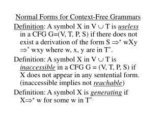
2. Normal Forms A normal form F for a set C of data objects is a form, i.e., a set of syntactically valid objects, with the following two properties: ● For every element c of C, except possibly a finite set of special cases, there exists some element f of F such that f is equivalent to c with respect to some set of tasks. ● F is simpler than the original form in which the elements of C are written. By “simpler” we mean that at least some tasks are easier to perform on elements of F than they would be on elements of C.

3. Normal Forms If you want to design algorithms, it is often useful to have a limited number of input forms that you have to deal with. Normal forms are designed to do just that. Various ones have been developed for various purposes. Examples: ● Clause form for logical expressions to be used in resolution theorem proving ● Disjunctive normal form for database queries so that they can be entered in a query by example grid. ● Various normal forms for grammars to support specific parsing techniques.

4. Normal Forms for Grammars Chomsky Normal Form, in which all rules are of one of the following two forms: ● Xa, where a, or ● XBC, where B and C are elements of V - . Advantages: ● Parsers can use binary trees. ● Exact length of derivations is known: S A B A A B B aab B B bb

5. Normal Forms for Grammars Greibach Normal Form, in which all rules are of the following form: ● Xa, where a and  (V - )*. Advantages: ● Every derivation of a string s contains |s| rule applications. ● Greibach normal form grammars can easily be converted to pushdown automata with no - transitions. This is useful because such PDAs are guaranteed to halt.

6. Normal Forms Exist Theorem: Given a CFG G, there exists an equivalent Chomsky normal form grammar GC such that: L(GC) = L(G) – {}. Proof: The proof is by construction. Theorem:Given a CFG G, there exists an equivalent Greibach normal form grammar GG such that: L(GG) = L(G) – {}. Proof: The proof is also by construction.

7. Converting to a Normal Form 1. Apply some transformation to G to get rid of undesirable property 1. Show that the language generated by G is unchanged. 2. Apply another transformation to G to get rid of undesirable property 2. Show that the language generated by G is unchanged and that undesirable property 1 has not been reintroduced. 3. Continue until the grammar is in the desired form.

8. Rule Substitution XaYc Yb YZZ We can replace the X rule with the rules: Xabc XaZZc XaYcaZZc

9. Rule Substitution Theorem: Let G contain the rules: XY and Y1 | 2 | … | n , Replace XY by: X1, X2, …, Xn. The new grammar Gwill be equivalent to G.

10. Rule Substitution Theorem: Let G contain the rules: XY and Y1 | 2 | … | n Replace XY by: X1, X2, …, Xn. The new grammar Gwill be equivalent to G.

11. Rule Substitution Replace XY by: X1, X2, …, Xn. Proof: ● Every string in L(G) is also in L(G): If XY is not used, then use same derivation. If it is used, then one derivation is: S … XYk … w Use this one instead: S … Xk … w ● Every string in L(G) is also in L(G): Every new rule can be simulated by old rules.

12. Conversion to Chomsky Normal Form 1. Remove all -rules, using the algorithm removeEps. 2. Remove all unit productions (rules of the form AB). 3. Remove all rules whose right hand sides have length greater than 1 and include a terminal: (e.g., AaB or A BaC) 4. Remove all rules whose right hand sides have length greater than 2: (e.g., ABCDE)

13. Removing -Productions Remove all  productions: (1) If there is a rule P Q and Q is nullable, Then: Add the rule P. (2) Delete all rules Q.

14. Removing -Productions Example: SaA AB | CDC B Ba CBD Db D

15. Unit Productions A unit production is a rule whose right-hand side consists of a single nonterminal symbol. Example: SX Y X A AB | a Bb YT TY | c

16. Removing Unit Productions • removeUnits(G) = • 1. Let G = G. • 2. Until no unit productions remain in G do: • 2.1 Choose some unit production X Y. • 2.2 Remove it from G. • 2.3 Consider only rules that still remain. For • every rule Y , where V*, do: • Add to G the rule X  unless it is a rule • that has already been removed once. • 3. Return G. • After removing epsilon productions and unit productions, all rules whose right hand sides have length 1 are in Chomsky Normal Form.

17. Removing Unit Productions • removeUnits(G) = • 1. Let G = G. • 2. Until no unit productions remain in G do: • 2.1 Choose some unit production X Y. • 2.2 Remove it from G. • 2.3 Consider only rules that still remain. For every rule Y , • where V*, do: • Add to G the rule X  unless it is a rule that has • already been removed once. • 3. Return G. Example: SX Y X A AB | a Bb Y T T Y | c

18. Removing Unit Productions • removeUnits(G) = • 1. Let G = G. • 2. Until no unit productions remain in G do: • 2.1 Choose some unit production X Y. • 2.2 Remove it from G. • 2.3 Consider only rules that still remain. For every rule Y , • where V*, do: • Add to G the rule X  unless it is a rule that has • already been removed once. • 3. Return G. Example: SX Y X A AB | a Bb Y T T Y | c SX Y Aa | b Bb T c X a | b Y c

19. Mixed Rules removeMixed(G) = 1. Let G = G. 2. Create a new nonterminal Ta for each terminal a in . 3. Modify each rule whose right-hand side has length greater than 1 and that contains a terminal symbol by substituting Ta for each occurrence of the terminal a. 4. Add to G, for each Ta, the rule Taa. 5. Return G. Example: Aa Aa B ABaC ABbC

20. Mixed Rules removeMixed(G) = 1. Let G = G. 2. Create a new nonterminal Ta for each terminal a in . 3. Modify each rule whose right-hand side has length greater than 1 and that contains a terminal symbol by substituting Ta for each occurrence of the terminal a. 4. Add to G, for each Ta, the rule Taa. 5. Return G. Example: Aa Aa B ABaC ABbC Aa ATa B ABTa C ABTbC Taa Tbb

21. Long Rules removeLong(G) = 1. Let G = G. 2. For each rule r of the form: AN1N2N3N4…Nn, n > 2 create new nonterminals M2, M3, … Mn-1. 3. Replace r with the rule AN1M2. 4. Add the rules: M2N2M3, M3N3M4, … Mn-1Nn-1Nn. 5. Return G. Example: ABCDEF

22. An Example SaACa AB | a BC | c CcC |  removeEps returns: SaACa | aAa | aCa | aa AB | a BC | c CcC | c

23. An Example SaACa | aAa | aCa | aa AB | a BC | c CcC | c Next we apply removeUnits: Remove A B. Add A C | c. Remove BC. Add BcC (Bc, already there). Remove A C. Add A cC (Ac, already there). So removeUnits returns: SaACa | aAa | aCa | aa Aa | c | cC Bc | cC CcC | c

24. An Example SaACa | aAa | aCa | aa Aa | c | cC Bc | cC CcC | c Next we apply removeMixed, which returns: STaACTa | TaATa | TaCTa | TaTa Aa | c | TcC Bc | TcC CTcC | c Taa Tcc

25. An Example STaACTa | TaATa | TaCTa | TaTa Aa | c | TcC Bc | TcC CTcC | c Taa Tcc Finally, we apply removeLong, which returns: STaS1 STaS3 STaS4 STaTa S1AS2 S3ATaS4CTa S2CTaAa | c | TcC Bc | TcC CTcC | c Taa Tcc

26. The Price of Normal Forms EE + E E (E) Eid Converting to Chomsky normal form: EEE EPE ELE EE R Eid L ( R ) P + Conversion doesn’t change weak generative capacity but it may change strong generative capacity.