Land Use Acreage BMPs Fertilizer Manure Atmospheric Deposition Point Sources Septic Loads

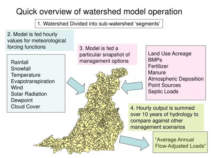
1. Rainfall Snowfall Temperature Evapotranspiration Wind Solar Radiation Dewpoint Cloud Cover Land Use Acreage BMPs Fertilizer Manure Atmospheric Deposition Point Sources Septic Loads Quick overview of watershed model operation 1. Watershed Divided into sub-watershed ‘segments’ 2. Model is fed hourly values for meteorological forcing functions 3. Model is fed a particular snapshot of management options 4. Hourly output is summed over 10 years of hydrology to compare against other management scenarios “Average Annual Flow-Adjusted Loads”

2. Phase 5 land segmentation isprimarily county-based • Some counties were divided to accommodate different rainfall patterns. Reasons why counties are a practical choice for segmentation: • Most counties are completely within a hydrogeomorphic region • BMP and Crop data are not known on a finer scale in most cases • Near the limit of computing capacity

3. Phase 5 river segmentation • Consistent criteria over entire model domain • Greater than 100 cfs or • Has a flow gage • Near the limit of meaningful data

4. A software solution was devised that directs the appropriate water, nutrients, and sediment from each land use type within each land segment to each river segment External Transfer Module Each land use type simulation is completely independent. Each river simulation is dependent on the local land use type simulations and the upstream river simulations.

5. Since this software is outside of HSPF, we can incorporate other features, for example, land use change or BMP change over the course of the calibration 1984-1999 External Transfer Module Land use change in the Patuxent Basin 1982-2002

6. Land Use Data Set Land cover data provided by the Regional Earth Sciences Application Center (RESAC) at the University of Maryland

7. Land Use Data Set 100% 80% 60% 40% 20% 0% RESAC also provided pixel by pixel impervious percentages Map of New York impervious percentages

8. The land use data set is a product of land cover, impervious percents, the US census of agriculture and an urban forecast and hindcast based on census data and density analysis Land Use Data Set U.S. Census of Agriculture 1982 1987 1992 1997 2002 + Urban Forecast and Hindcast +

9. Construction Land Use • Originally tried to use satellite “BARE” classification

10. Construction Land Use • Tied to Change in Impervious • Have impervious 1990 and 2000, gives change per year • Assume that the average construction time is 1 year • Assume that the ratio of disturbed acreage to new impervious is 10:1

11. Comparisons with MD and VA • MD has 128,000 permitted disturbed acres in 1999 and 74,000 in 2004 • Model has 80,000 • VA estimated 30,000 to 50,000 statewide • Model has 118,000

12. Comparison with MD data

15. A program was written to automatically calibrate the hydrology for all stations and land segments. This plot shows average NS efficiency for all 284 calibration stations versus iteration The calibration becomes stable after approximately ten iterations

16. Sediment Pathway in Phase 5 Edge of Field BMP Factor 1. Sediment processes are simulated on the land surface resulting in an Edge-Of-Field sediment load. 2. A time series of Best Management Practice (BMP) factors is applied based on available data. 4. A delivery factor based on local geometry is applied (see below), resulting in the Edge-Of-Stream load. Land Acre Factor Edge of Stream Delivery Factor 3. A time series of land use acreage factors is applied. 5. Processes of deposition and scour are simulated in the stream, resulting in concentrations that can be compared to observations. In Stream Concentrations

17. Sediment Pathway in Phase 5 Edge of Field BMP Factor There are two calibration points in this simulation. 1. Edge-of-Field loads are calibrated to expected values according to land use type or other data. 2. In-stream concentrations are calibrated where data are available (approximately 150 stations) Land Acre Factor Edge of Stream Delivery Factor In Stream Concentrations

18. Forest Harvested Forest Natural grass Extractive Barren Pervious Urban Impervious Urban Pasture Poor Pasture Hay High till with manure High till no manure Low till with manure Needed EOF targets for 13 land uses Agriculture Other The National Resources Inventory program of the NRCS provided the CBP with estimates of Pasture and Crop by county, based on an aggregation of point measurements applied to RUSLE. No such data available. Other data sources or analyses necessary. 13 land uses are being used for the sediment calibration. The other land uses are identical to one of the 13 for sediment purposes.

19. Pasture => Pasture Poor Pasture => 9.5 * Pasture Hay => 1/3 Crop (P4 NRI) High till with manure => 1.25 * Crop High till no manure => 1.25 * Crop Low till with manure => 0.75 * Crop Needed EOF targets for 13 land uses Agriculture Land use % of model Target relative to NRI estimate 9% 0.05% 7% 4% 1% 4% NRI provided direct estimates for Pasture. Poor Pasture is pasture that is heavily trampled near streams. It is a small land use that exports at a high rate. NRI provided estimates for Hay for the phase 2 model. The estimates were generally 1/3 of crop for that data set, so the proportion was kept. Low till is generally 40% lower than High Till, so that ratio was applied with an average value of the NRI estimate.

20. Forest Harvested Forest Natural grass Bare Extractive Pervious Urban Impervious Urban Needed EOF targets for land uses not included in the NRI estimates Other Forest: NRI estimates exist for phase 4 for the Chesapeake Bay watershed. Use these where available. For simulated areas outside of the Chesapeake Bay watershed, use USLE populated by GIS estimates of factors. Ratio the results to that the range is equal to the range for the Chesapeake Bay Watershed Harvested Forest: Bare ground erosion rates of forest soils are three to four orders of magnitude greater than base forest erosion rates, but current practice in Mid-Atlantic Region does not reduce forests to bare ground generally. Use 3.4 t/ac/yr as target rate, which is one order of magnitude greater than the average base forest rate. 65% 0.65% 0.65% 0.52% 0.11% 7.1% 1.2% The above land uses are discussed on the following pages

21. Forest Harvested Forest Natural grass Bare Extractive Pervious Urban Impervious Urban Needed EOF targets for land uses not included in the NRI estimates Other Natural Grass: Similar to Pasture and probably confused with it in a GIS analysis. Use the NRI pasture numbers by county Bare: This is simulated as a construction land use with acreage based on the local annual change in urban land. Estimates of sediment export from construction sites in the literature range from 7-500 tons/ac/year. An ‘average’ value of 40 tons/ac/year is assumed. Extractive: Active mining operations are permitted at low rates of sediment export ≈ 0.16 tons/ac/year. Abandoned mines have waste piles and non-vegetated area that act more like construction sites. With high uncertainty and but low overall load assume that extractive areas have the relatively high load of 10 tons/ac/year 65% 0.65% 0.65% 0.58% 0.11% 7.1% 1.2%

22. Forest Harvested Forest Natural grass Bare Extractive Pervious Urban Impervious Urban Needed EOF targets for land uses not included in the NRI estimates Other Urban: Post-construction urban sediment loads is primary due to channel erosion from increased concentrated flow from impervious surfaces. National Urban Runoff Program data are several decades old limited in applicability. Large amounts of data were collected under the phase I stormwater regulations, but studies by Penn State and University of Alabama have not been able to make predictive models from the collected data. Use Langland and Cronin (2003) estimates of urban EOS erosion rates by land use category. (following page) 65% 0.65% 0.65% 0.52% 0.11% 7.1% 1.2%

23. Urban Sediment Targets Sediment load for several urban land use types were compiled for sites in the mid-Atlantic and Illinois. Langland and Cronin (2003) When plotted against ‘typical’ impervious percents for those urban land use types, the relationship is striking. By setting pervious urban at the intercept and impervious urban at the maximum, the land use division within each particular segment determines the overall load according to the above relationship.

24. Wash off Generation Attachment Rainfall Detachment Land Sediment Simulation Detached Sediment KSER KRER AFFIX NVSI Soil Matrix (unlimited) 4 parameters, 1 target

25. Reduce the parameter set by enforcing calibration rules Calibration Goal - Zero Detached Sed after Large Storms Sediment transport has a natural hysteresis whereby storms that happen soon after other storms tend to have lower in-stream concentrations than the antecedent storms. This effect is negligible after 30 days. It is unclear if this is a river or land surface process, but there is no mechanism in the river simulation in HSPF to enforce this. vanSickle and Beschta (1983) Allen Gellis (personal communication) Surface Runoff Detached Sediment Storage Washoff To make this happen, AFFIX must be appropriately set, NVSI must be significant, and KRER must be small enough relative to KSER to avoid detached sediment buildup

26.  Basic HSPF equation where S = storage Rule 1:Set AFFIX so that Detached Sediment storage reaches 90% of its max in 30 days  At dS/dt = 0  For storage = 0 at t = 0 Solve equations so that detached storage versus time has the desired properties of reaching 90% of asymptote in 30 days. AFFIX = 0.07673

27. Generation Rainfall Detachment Rule 2 – Generation makes up significant portion of Detached Sediment Detached Sediment Generation and Rainfall Detachment can both generate detached sediment. The proportion of the detached sediment made up of generation is positively related to the amount of hysteresis in the simulation. KRER NVSI Soil Matrix (unlimited) • NVSI = [significant fraction] * target load

28. Detached Sediment (reservoir available for washoff) Wash off KSER Rainfall Detachment KRER Attachment Generation AFFIX NVSI Soil Matrix (unlimited) Rule 3 – KRER is a percentage of KSER Excessive KRER relative to KSER will lead to a buildup of detached sediment, so that KRER is a percentage of KSER

29. Detached Sediment Generation Wash off KSER Rainfall Detachment Attachment KRER AFFIX NVSI Soil Matrix (unlimited) Strategy: Reduce the Parameter Set 1. Fix AFFIX 2. Assume ratio of NVSI : EOF target 3. Assume ratio of KSER : KRER 4. Adjust KSER to meet target 1 parameter, 1 target Make several runs with different ratios (#2, 3)

30. More hysteresis Greater effect of plowing Different scenarios make little difference on the correlation of simulated and observed concentrations Correlation of sediment concentrations for each of 8 scenarios

31. More hysteresis Greater effect of plowing Average detached storagedecrease withDecrease of NVSI ratio and Increase of KSER/KRER ratio Average detached storage for each of 8 scenarios

32. In Stream Concentrations Land-to-Water Delivery Factors Edge of Field BMP Factor Edge of Stream Land Acre Factor Delivery Factor Land uses are not evenly distributed around a segment and some segments are larger than others. A method to assign a differential delivery factor for each land cover class and segment is shown on the following slide.

33. Sediment delivery factors by land use and segment Several publications were found that relate sediment delivery to watershed size. The most appropriate one was judged to be the SCS method: DF = 0.417762 * Area -0.134958 - 0.127097 The delivery factor needed for the phase 5 model is from land cover pixels to the stream, not to the watershed outlet, so it is not appropriate to use the size of the watershed. To generate a deliver factor for each land use, the average distance of that land use to the stream was used as radius of a circle. The area of that circle was used to calculate the delivery factor. To illustrate this approach, suppose a land use type that is scattered throughout a segment were gathered into a single area, but the distances to the stream were preserved. The average delivery of that cluster would be roughly equal to the average delivery from a circle with a center that was co-located with the center of mass of the land use.

34. River Calibration

36. Outflow Inflow Deposition Scour River Cohesive Sediment Simulation Suspended Sediment Bed Storage (unlimited)

37. Deposition River Sediment Simulation Bed Storage (unlimited)

38. Scour River Sediment Simulation Bed Storage (unlimited)

39. River Sand Simulation Adjustments are then made to the bed depth

40. All rivers segments upstream of a calibration point have identical parameters For nested rivers, this applies only to rivers downstream of any upstream gages. Remington Robinson Rappahannock Calibration Rules 1

41. Uncalibrated

42. Stau 97 percentile Ctau 93 SW .001 inches/sec CW .0001 CM = 1 lb/ft^2/day SM = 1 KS = .003 empirical ES = 4 High flow in the ballpark, but low flow is a problem. Lowest concentrations are mostly VSS, which is not yet simulated and are at LOD in the observed

43. Stau 97 Ctau 93 SW .001 CW .0001 CM = 1 SM = 1 KS = 3 ES = 3 To deal with the lack of VSS in the simulation, use SAND to make the low concentrations work out. This can be easily reversed when VSS are simulated

44. Stau 99 Ctau 96 SW .001 CW .0001 CM = 1 SM = 1 KS = 3 ES = 3 Reduce the frequency of scour to deal with over-simulation

45. Stau 99 Ctau 96 SW .001 CW .0001 CM = .5 SM = .5 KS = 3 ES = 3 Reduce the effect of scour to deal with over-simulation

46. Stau 99.5 Ctau 98 SW .001 CW .0001 CM = .5 SM = .5 KS = 2.8 ES = 3 Tighten up the simulation

47. Issues with simulation • Low values dominate the CFD, but they are not meaningful from: • A load standpoint • An accuracy of observation standpoint • Simulation standpoint (no VSS) • Flow not perfectly calibrated • If peak is missed by a day, then the concentration simulation should not match the observed.

48. If simulated or observed value is below 10 mg/l set it to 10 mg/l. Check simulation for 24 hours before and after observation and set simulated value to point closest to observation. ‘Windowed’ comparison Of the highest observed and simulated peaks at all calibration stations, almost as many peaks occurred one day apart, but few occurred on two days apart One day apart – 83% of the same day figure Two days apart – 19% of the same day figure

49. Reported Error I

50. Stau 97 Ctau 93 SW .001 CW .0001 CM = 1 SM = 1 KS = .003 ES = 4 Starting point