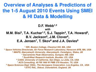
Overview of Analyses & Predictions of the 1-5 August 2010 Events Using SMEI & HI Data & Modelling

1. Overview of Analyses & Predictions of the 1-5 August 2010 Events Using SMEI & HI Data & Modelling D.F. Webb1,2 with M.M. Bisi3, T.A. Kuchar1,2, S.J. Tappin4, T.A. Howard5, B.V. Jackson6, J.M. Clover6, E.A. Jensen7, T. Skov8 and J.A. Davies9 1 ISR, Boston College, Chestnut Hill, MA, USA 2 Space Vehicles Directorate, Air Force Research Laboratory, Hanscom AFB, MA, USA 3 IMAPS, Aberystwyth University, Aberystwyth, Ceredigion, Wales, UK 4 Sacramento Peak Observatory, Sunspot, NM, USA 5 SouthWest Research Institute, Boulder, CO, USA 6 CASS, University of California, San Diego, La Jolla, CA, USA 7 ACS Consulting, 40 FM 1960 W PMB 370 Houston, TX, USA 8 Space Sciences Dept/ SSAL, The Aerospace Corporation, Los Angeles, CA , USA 9 STFC RAL, Didcot, Oxfordshire, England, UK

2. Observations of ICMEs using SMEI • SMEI saw ICME material mainly on 3 August 2010 and predictions were made using two models from the direct images which are routinely used for forecasts. Both models predicted Earth arrival about 22:00 UT on 3 August. This is slightly later than the shock, but before MC1 on 4 August. So, the SMEI predictions seem to fit well with the discussions of the shock, sheath, and both MCs. • The ICMEs’ brightnesses were moderate and the observations considered of “Good” quality. Speeds of 850 km s-1 and 974 km s-1 were calculated from the Tappin-Howard (T-H) and tool models, respectively. • A shock occurred at the ACE spacecraft on 2 August at 17:00 UT. Kp was ‘double peaked’, reaching 7 early on 4 August and then again 6 later the same day. The Dst index reached -77 nT. SMEI observed high auroral emission from 3 August at 19:30 UT, or just after shock arrival, and throughout 4 August. The aurora was over in the gap between images on 4 August at 22:30 UT and 5 August 05:30 UT (see next movie). • The large CMEs during 1-5 August were predicted several hours in advance by both models and 3-D reconstructed by the T-H model.

3. Observations of ICMEs with SMEI Data SMEI observed two arc segments during Aug. 3-4 (DOY 215-216). They were first observed in SMEI on Aug. 3, 09:12 UT, and over a duration of >20.5 hr. The main arc was over the ecliptic north pole and NNE, and another segment was to the ESE. AFRL processing – Fisheye projection: Aug. 3-4. Shows both arcs and the aurora

4. Observations of ICMEs with SMEI Data If these two arcs were part of one ICME arc it would have extended over >160°. But the elongation-time plot suggests they are two separate structures, with the eastern one much farther out. These arc measurements are: East: PA = 102°; Aug. 3, 15:08 - 18:31 over elongations 82.8° – 84.1°. North: PA = 357°; Aug. 3, 13:51 – 17:14 over elongations 47.3° – 55.3°. Webb SMEI Aug10 UK2011 Wks

5. Forecasting Earth Arrival of CMEs Using SMEI Data • These forecasts were made with either of the two models: • - A SMEI tracking ‘tool’ developed for the Air Force Weather Agency (AFWA); • - The Tappin-Howard (T-H) model (e.g. Howard and Tappin, Space Weather, 2010). • For each forecast we record: • - the predicted speed and time of arrival (ToA) of the ICME at 1 AU; • - the time that the forecast was made. • Afterwards we also record: • - the launch information from surface and coronagraph observations; • - the subsequent circumstances at L1 (ACE in this case). • A probability of Earth impact is added based on the calculated CME-Sun-Earth angle: • - For the T-H model a hit or miss is based on whether or not Earth will cross • the calculated CME area; • - Probability is based on statistical survey of ~ 20 SMEI events measured • during 2003-2006. • The T-H predictions were compared with actual measurements by in-situ spacecraft and geomagnetic activity! • The following slides briefly explain how the tool and T-H models work, and the arrival-time predictions that were made using these models with the SMEI white-light data.

6. SMEI Tracking Tool - Measure & Plot CME Trajectory Left:A CME’s leading edge is tracked on successive running-difference images/movies using the SMEI program. Each point has an elongation (angular distance from Sun center) vs. time coordinate. Right: All resulting points are then plotted. The curve assumes the CME travels at a fixed radial direction and speed. Free parameters are its speed, Sun-Earth angle, and launch time; these are determined from least-squares fit to elongation-time data.

7. SMEI Tool Plotting Results • Fitting routine assumes constant velocity from launch point • Can input LASCO measurements for more accuracy • Routine output (example of 27 January 2007 shown here) ASSIGNING DEPARTURE TIME = 25.41 ESTIMATES: CME TRUE SPEED = 847.8 km s-1 ANGLE FROM SUN-EARTH LINE = 42.2° ARRIVAL TO 1 AU = DOY 027 at 11:04 UT RELATIVE SOLAR LONG., LAT. = -28.0° and -32.9° respectively Test operational interface for SMEI CME/ICME Measurements (AFWA)

8. The Tappin-Howard (T-H) Model The T-H model produces an estimate of CME geometry and kinematics by comparing leading edges measured in heliospheric image data with those from simulated CMEs. Thomson scattering effects are accounted for. Shell • First, a basic structure is chosen: • A spherical arc or a solar centered (shell) • Then independent combinations of: • Speed • Distance • Central Latitude • Central Longitude • Latitude Width • Longitude Width • Distortion Parameter • Are combined to produce CME simulated images from which leading edges are produced relative to a fixed observer. Observer Sun Distortion Observer Sun [Tappin & Howard, 2009]

9. SMEI Prediction Results for August 2010 SMEI Tool Results: Relative Solar Long., Lat. = 37.6°, 50.5° respectively CME Speed = 974 km s-1 Angle From Sun-Earth Line = 59.8° Arrival Time at 1 AU = 3 August at 23:04 UT Time Prediction Made = 3 August at 18:05 UT Advance Warning Time = 5.0 hr. T-H Model Results: Onset at the Sun = 1 August 20:00UT (± 0.7 days) Central location = 28°W 23°N [± ( 15°,12°)] CME Speed = 850 km s-1 (± 180 km s-1) CME Size = 43° (± 9° - EW), 23° [± 8° (NS)] Closest approach to Earth = 3 August 22:30 UT (± 30min) 50% chance of a hit Time Prediction Made = 3 August 18:0 2UT Advance Warning Time = 4.5 hr.

10. STEREO-SECCHI Movies (RAL): mid-1 to 3 August • HI-A from Aug. 1, 1200 to end of Aug. 3 • HI-B from Aug. 2 to end of Aug. 4 • RH Features M and L noted on images • CORs and HIs show lots of activity before 1 Aug., and some of this goes to the South – particularly in ST-B imagery (see SMEI 3-D reconstructions later) L M M?

11. August 2010 CME Table CME Time Name Flare J-plots 1 AU -1 30,0700 Flare 0 ? --- ST-B halo VEX, ST-B? E70 1 1, 0300 Flare 1 B4 M E30 ? 2 1, ~0730 Flare 2 C3 L E50 Earth 3 1, 0730 Fil 1 --- “N”,A? N-most fil. Earth? 4 1, 1600 Fl/Fil 2 B4 B sm. W fil. Earth 5 1, 2100 Fil 3 --- --- S-most fil. ?

13. 3 August 2010 T-H HI2A Fit Results HI2A(a) – 3 Aug; 01:50 UT HI2A(b) – 3 Aug; 01:50 UT ST-B ST-A Earth HI2A(c) – 3 Aug; 01:50 UT SMEI – 3 Aug; 08:50 UT (a) (Closest approach) MC1 MC2 (b) (c) • Will hit Earth • Miss 18°; hit prob. 45% • Miss 9°; hit prob. 65%

14. 3 & 6 August 2010 T-H SMEI Fit Results SMEI– 6 Aug; 03:54 UT SMEI– 3 Aug; 08:50 UT Aug. 3: Will hit Earth Aug. 6: Miss 10°; hit prob. 60%

15. Note that the HI2 (a) and (b) fits and the SMEI Aug. 3 fit, with locations all shown as early on Aug. 3, seem more or less consistent with the ENLIL runs given in Dusan’s talk. • Besides the Aug. 3 SMEI front there is another later event to the west of Earth, shown on Aug. 6. Both events are only detected by SMEI near Earth, and their locations are shown in the distance-time plot. • Next are shown ENLIL views early on Aug. 3; note the 3 ICME fronts, with one close to the Sun-Earth line like SMEI and another to the east like the HI2A (a) shell in the T-H run. Dusan’s HI2B simulation shows the densest material to the north, as with the (a) and (b) T-H runs shown here (see Dusan’s talk). This gives us some confidence with the geometry, shapes, and sizes of the CME fronts shown here. • Taken together one interpretation is that the SMEI, HI2 (a) and (b) fronts and RH’s feature “M” are part of the same ICME that arrives at L1 late on Aug. 3. Tim Howard thinks HI2A front (a) and SMEI see the shock sheath, HI2A (b) is the LE of MC1, and HI2A (c) is the LE of MC2.

16. ENLIL-Synthetic W-L Images – HI-2 (Triangulation) From D. Odstrcil slides

17. Recent SMEI 3-D Reconstruction Results UCSD SMEI 3-D reconstructions of the August 1–5 period. LEFT: On Aug. 4, 00 UT note dense structures near Earth, beyond ST-B, and approaching 1 AU between ST-A and Earth (west of Sun-Earth line) in the ecliptic view. RIGHT: a high resolution meridional view. At first we thought the dense material to the South was noise, but the STEREO data suggests this may be real and the result of earlier activity, perhaps on July 30 or 31. Ecliptic View Meridional View

18. Latitudinal Comparison with STEREO HI-A Material flowing out more slowly North of the ecliptic in the HI-A images is likely reconstructed by SMEI as shown here in the meridional cut (right) inside of 1 AU on Aug. 4, 00 UT.

19. Recent SMEI 3-D Reconstruction Results Movies of the recent UCSD SMEI 3-D density reconstructions during the 2-6 Aug. period. The ecliptic view is on the left and the meridional view on the right. Note the double density peaks. We plan to eventually derive masses and energies of this material.

20. Cross-correlation of SMEI reconstructed & in-situ densities • Lower 3-D resolution: • 6.7º in latitude and longitude resolution • 0.50-day temporal resolution  CME onset • Higher 3-D resolution: • 3.3º in latitude and longitude resolution • 0.25-day temporal resolution • Has a higher correlation • Note that the first peak above resolves into two peaks: late on Aug. 3 (shock?) and midday Aug. 4 (MC1; 2?).  CME onset Masayoshi

21. FR fits by Tamitha Mulligan Skov Time series plots showing FR fits for VEX and STB.  Fit at ACE is LH and fits at VEX and STB are RH.  When I try to fit the VEX and STB observations with a LH rope, the solution is VERY non-force-free.  Since Liz's model is a force-free Bessel function, I’ve asked her to see if she can fit the ropes at VEX and STB.  Her results maybe will show a decent fit with a RH structure and a bad one with a LH structure  the MC2 structure at ACE/Wind is not the same flux rope (M3) as seen at VEX and STB.

22. FR fits by Tamitha Mulligan Skov (& Liz Jensen)

23. FINI Questions?

24. Observations of ICMEs with SMEI Data Tappin processing – Aitoff projection: Aug. 3-4. Shows the northern arc and aurora well

25. ICME SMEI Tracking Tool Developed for AFWA Improve forecasts by using heliospheric imaging measurements for assimilation into an existing forecast model (e.g. the HAFv2 model). Forecast timeline: • Issue a forecast (e.g. HAF) • Analyze SMEI imagery • Compare with observation • Adjust forecast • Iterate this process SMEI HAFv2

26. The Tappin-Howard (T-H) Model The Model is run in 2 stages: Stage 1 converges to a solution containing a unique combination of each of the parameters. Along with a fixed direction and structure, this also produces a single speed, allowing only for a constant speed ICME. Stage 2 considers smaller subsets of data measurements, leaving the direction and structure fixed, but allowing the speed parameter to vary from one combination to another. Other parameters can be allowed to vary as well. Employing Stage 2 allows us to monitor small changes in the kinematics of the ICME, particularly variations in speed and acceleration. D t D t [Tappin & Howard, 2009]

27. Preliminary Flux-Rope Modelling Fits (OMNI Data) • 3 August 2010 ICME properties: • Weak, over-expanding rope with little axial field; • Start time: 18:00UT; • End time: ~10:00UT (on 4 August); • Axis orientation: GSE z-direction (South); • Handedness: right handed. Bessel function solution (red): Clock Angle: -86° (+ from GSEY to GSEZ, in YZ-plane); Cone Angle (from GSEX): 77°; Impact parameter: 2% (dawn side); Magnetic Field: 10 nT. Mulligan (non-force-free) solution (green): Clock Angle: -151°; Cone Angle: 134°; Impact parameter: 50% (dusk side); Magnetic Field Axial: 22 nT; Magnetic Field Toroidal: 20 nT. (T. Mulligan Skov & L. Jensen)