Download

1 / 62
620 likes | 762 Views
The creation of magnetic structures from velocity shear (Constraints for the solar dynamo) Nic Brummell Applied Mathematics, University of California Santa Cruz Geoff Vasil, Kelly Cline JILA/APS, University of Colorado Lara Silvers, Mike Proctor DAMTP, University of Cambridge, UK.

E N D
The creation of magnetic structures from velocity shear (Constraints for the solar dynamo) Nic Brummell Applied Mathematics, University of California Santa Cruz Geoff Vasil, Kelly Cline JILA/APS, University of Colorado Lara Silvers, Mike Proctor DAMTP, University of Cambridge, UK UCSD Feb 2009
Major puzzle: solar magnetic activity cycle Solar magnetic activity is VARIABLE but remarkably ORDERED. How does it work? A DYNAMO! But how does the dynamo work?
Theories driven by observations Things we know surprisingly well -- solar interior structure(thanks to helioseismology) Solid body rotation in the core Interface layer – theTACHOCLINE Differential rotation in the convection zone
Large-scale dynamo: Theory Existing poloidal field is stretched by latitudinal (and/or radial) differential rotation into the toroidal direction – an -like mechanism Strong toroidal field rises due to magnetic buoyancy and, under the influence of global rotation, twists into the poloidal direction – an a-like mechanism
Strong toroidal field rises as structures? MAGNETIC BUOYANCY: the standard explanation Magnetic field exerts a magnetic pressure (Lorenz force JxB can be split into pressure and tension ) Concentrated B contributes to the total pressure Isothermal pressure balance implies density lower in tube Pg = density*temperature Outside: Pt = Pg1 Inside: Pg2 = Pt-Pm Pm ~ B2 => Pg2 < Pg1 densityinside < densityoutside
Magnetic buoyancy instabilities 101 End result: Magnetic GRADIENTS that are important! (gradients in the direction of gravity)
Large-scale dynamo: intuitive picture • Generation/shredding of magnetic field • Transport of magnetic field from CZ into tachocline -- TURBULENT TRANSPORT OF B ? • W effect: Conversion of poloidal field to toroidal field -- DIFFERENTIAL ROTATION -- ORIGIN ? • Formation of structures and magnetic buoyant rise -- MAGNETIC BUOYANCY / SHEAR ? • a mechanism: Regeneration of poloidal field -- ROTATION, TURBULENT u, b CORRLNS?? • Recycling/breakdown of field • Emergence of structures STUDY ELEMENTS OF THE DYNAMO
Heavily dependent on the tachocline Boundary layer between • the convection zone (differentially rotating) • the radiative interior (solid body rotation) Layer (plus sub-layers?) of • strong radial shear • weaker latitudinal shear Almost certainly threaded with magnetic field • weak poloidal? • strong toroidal? We wish to examine, via fully nonlinear MHD simulations: • the interaction of velocity shear and weak background (poloidal) magnetic fields. • the production of strong (toroidal) magnetic fields by the shear • magnetic structures produced • any magnetic buoyancy instabilities of the magnetic configuration • the nonlinear evolution of the system
Cons of mass Mmm … nonlinearity! pressure rotation Cons of mom buoyancy advection tension forcing diffusion Mmm … nonlinearity! Cons of energy Compression Advection Ohmic & viscous heating diffusion Mmm … nonlinearity! Induction Induction diffusion magnetic pressure Compressible MHD equations (Navier-Stokes + induction) So … how does it work?
z=0 Layer 1 : Unstable m = m1 (=1) z=1 Layer 2 : Stable m=m2 (>1.5) z=zmx Local simulations of elements of the dynamo e.g. Brummell, Clune & Toomre, 2002 Full compressible MHD (poloidal/toroidal) DNS Cartesian Pseudospectral / finite-difference Semi-implicit HIGHER Rq, Re, Pe, LOWER Pr than global sims (resolves from diffusive scale UP) Thermal diffusivity k=k(z) ( not k(r,T:x,y,z) ) : Ck(layer1)/Ck(layer2)=(m2+1)/(m1+1) “Stiffness”, S = (m2-mad)/(mad-m1)
So … how do we solve these? Blue Gene/L Fastest machine in the world! ~ 213,000 cpus 596 Tflops peak, 478 sustained
(a) Latitudinal shear: Bf = q latitude + Bf f longitude dVf/dq Bq (b) Radial shear: Bf + Z = depth f longitude Br dVf/dr The mega effect Interaction between shear (gradients) in the azimuthal velocity and the poloidal magnetic field produces strong toroidal magnetic field.TWO POSSIBILITIES: (the usual) (the not-so-usual)
radial latitudinal Good reasons for the not-so-usual … But really interested in gradientsfor magnetic buoyancy: ∂t BT = BP• δΩ + … , δΩ = r*sin(ϴ) ∇Ω Differentiate MDI observational results: Therefore reasons: • Radial shear is stronger • Need radial gradients for magnetic buoyancy • Some radial component likely • Horizontal scale selection - better option?
Case (a): Latitudinal shear (a) Latitudinal shear: Bf = q latitude + Bf f longitude dVf/dq Bq
By + Model: Localised latitudinal velocity shear Mimic some properties of the tachocline : • Use a convectively stable layer • Force* a velocity shear in both the vertical (z) and one horizontal (y) direction. e.g. U(y,z) = f(z) cos(2 p y/ym) where f(z) is a polynomial function chosen to confine the shear to a particular layer between zu and zl (and to be sufficiently continuous) • Shear flow is hydrodynamically stable Then add an initial magnetic field: B0 = (0, By , 0) withBy = 1 * Add term in the equations that induces desired flow in absence of magnetic effects
Increasing Rm: Magnetic buoyancy instability A more interesting movie! • Instability • Cyclic activity • Two out-of-phase sequences of identical but oppositely-directed magnetic structures. • Broken the y-reflectional symmetry
Latitudinal shear: conclusions First demonstration that buoyantly-rising strong (toroidal) magnetic structures can be spontaneously generated by the action of shear on a background (poloidal) magnetic field. BUT … Radial gradients stronger => stronger toroidal field? Currently the structures have scale of the latitudinal shear = BIG (too big) SO … Try radial gradients?
Uo(z) BZ + Strong layer of Bx created BX Forced Initial Final So consider … Case (b): Radial shear One might expect: Yes! … but turns out that this is much harder to make work than you might think!
Radial shear: Magnetic buoyancy Magnetic buoyancy instability: volume rendering of abs(B) 768^3 200,000 cpu hours … yikes! Measured Taylor microscale Reynolds number ~ 30 Pm=0.625
Radial shear: Looks good, but problems … Bx z Time Not much flux transport. Inefficient
Radial shear: Problems The forcing required to make this work is HUGE! Target velocity of forcing is about Mach 15! Yikes! If you run the same case without magnetic field, keeping the same large forcing, get some serious Kelvin-Helmholtz turbulence! WHY SUCH A LARGE FORCING? RE-CAST THIS QUESTION …
Is the tachocline this strongly maintained? Is itmaintained by external processesindependent of tachocline dynamics? (USUAL POV) Ormust maintaining processestake into account internal dynamics? (UNUSUAL POV) Must the tachocline be STRONGLY MAINTAINED against the tachocline dynamics? In other words: is the shear we oberve the target shear of a a particular forcing or a modified shear returned at the end of a complex nonlinear process? Two simple 1-D analytic models to try and answer this question: Completely unmaintained shear Weakly maintained shear If these don’t work in some sense, then answer is shear is strongly-maintained. We evaluate under what conditions a magnetic buoyancy instability can manifest itself …
Stability condition Condition for instability (Newcomb 1961): around a mechanical equiilibrium where N is the Brunt-Vaisalla frequency can be recast as Thermodynamics: Adiabatic => N = N0, const. (Reasonable but we’ll come back to this) Note that NONE of this is really valid in our case, of course! : • No mechanical equilibrium : background state evolves! • Shear flow on top BUT look to see if this is even CLOSE to being satisfied as an indication of LIKELIHOOD of magnetic buoyancy …
Model 1: No maintenance of the shear (slow rundown) • things happen fast so can ignore complex nonlinear back reactions on the shear • maintainence of shear independent of tachocline dynamics Examine time-dependent buildup of the toroidal field: No forcing, linearisation … Induction eqn: stretching production of tor field by shear on pol field Momentum eqn: linear back reaction on the shear Easy: assume background density const (but don’t have to) Initial conditions: Bx=0 and a given profile u=U0(z) => solutions => Alfven wave dynamics
Alfven wave dynamics Analytical: constant wave speed U(t,z) Initial condition: U0 = tachocline-like jump, Magnitude U0, width z Bx(t,z)
Full 3D simulations: Failures :( We have plenty of examples of the types of dynamics we describe … Forcing not large enough: System heads to diffusively-balanced state plus Alfven waves. U Bx
Amplitude of Bx Bx grows but saturates. Really is just superposition of two waves, and only “grows” when they are interfering. Bx grows whilst interference is in shear zone, then halts in the constant parts of U0 i.e. Bx grows until i.e. grows for Alfven crossing time tA across half layer. Two phases of dynamics: • “Growth” (actually interfering waves) for t < tA Bx grows linearly like and u ~ U0 • “Wave propagation” for t > tA with Can Bx get big enough for magnetic buoyancy instability? Linear growth up to a saturation max value
Model 1: Instability? Estimate gradients of Bx from this amplitude simply as (Bx(max)-0)/z/2 Differentiate Plug into mag buoy instability condition (adiabatic version) or Richardson number of forced flow, Ri < z/H Small!! Need highly shear unstable original flow for possibility of mag buoy instabilities!! Rule of thumb: Ri < 1/4 => turbulent shear Tachocline Ri ~ 1000? Maybe NO maintenance is not enough! Try some weak maintenance? => Model 2
Model 2: Weak maintenance of the shear Examine time-independent state weakly forced state Momentum Induction Integrate, combine and figure out some bounds … => estimate of max amplitude of toroidal field Pm = magnetic Prandtl number Magnetic energy bounded by the kinetic energy of the the forcing (but with Pm factor) Stability? Ri/Pm < z/H or Ri < Pm . z/H EVEN WORSE!
Conclusions: UNDER THE ASSUMPTIONS -- WEAK OR NO MAINTENANCE OF SHEAR => SHEAR INDEPENDENT OF TACHOCLINE DYNAMICS then to get magnetic buoyancy instabilities NEED -- large forcing (large = hydrodynamically unstable) -- or high Pm We have confirmed these simple ideas with massive numerical simulations! (buoyancy found at small Pm for large forcing, or at large Pm for small forcing) Ultimate conclusion: The maintenance of the tachoclineneeds to know about tachocline dynamics. In other words,we have to do a more self-consistent problem. Pm=4000 U0=1.2
Radial shear: Thoughts Action of radial shear on radial field -- conclusions: • For magnetic buoyancy to occur, must stretch the field fast enough that Alfven waves cannot radiate the magnetic energy away. • Simple models, confrmed by numerical experiments, show that this requires a very strong initial/target shear -- one that is probably hydrodynamically unstable (or a high Pm which is not valid for the Sun). • The models assumed that the tachocline dynamics and the processes that maintained the tachocline itself were independent. At this stage we concluded that this must not be true and a more holistic, more complicated model of tachocline dynamics was needed. • We had pondered one quirky caveat in this work however, and had only speculated on it’s effect. That was the possibility of a DOUBLE-DIFFUSIVE INSTABILITY.
Double-diffusive instabilities 101 In the presence of TWO components that affect the density, can have an instability even if the overall density stratification is convectively stable. e.g. ocean water: warm salty water overlying cooler fresh water IF the diffusivity of the stabilising component is much LARGER than that of the stabilising component, can have instability: Parcel perturbed upwards should return downwards due to temperature deficit but this diffuses away quickly, and so continues upwards due to relative freshness. warm salty cool fresh Overall density stratification stable Thermal stratification stabilising Salinity stratification destabilising
Double-diffusive magnetic buoyancy In the earlier work , we assumed that the thermodynamics adjusted adiabatically. If we assumed that the thermal diffusivity was sufficiently large, then we could re-do the work assuming that the adjustment was isothermal. Now we have to include the diffusivities via the ratio (Note: not Pm!) This is equivalent to looking for double-diffusive instabilities in this system. AdiabaticIsothermal Clearly, if is small, then this inequality is more likely satisfied.
Double-diffusive instability Two simulations differing only in the thermal diffusivity and therefore Fixed magnetic and viscous diffusivity (=> Prandtl number changes) Lower is unstable!
Double-diffusive instability Fluctuations are induced in B and w
Double-diffusive instability Added complexity: Since this is not a bifurcation about a static equilibrium but rather one about a dynamically-evolving background state, there is a condition on the growth rate as well as just a “Rayleigh number” criterion (Ratot~RaT-RaB) Growth rate must be faster than the evolution of the background for instability to manifest. Background evolves on the Alfven timescale of the background field, so now dynamics depends on background field strength! Instability occurs weaker and higher up. We are still working on the nonlinear evolution of this instability …
Conclusions Solar boundary layer -- the tachocline -- essential for solar dynamics. Dynamics of the tachocline very mysterious. In terms of generating buoyant magnetic structures: • TYPE 1: Latitudinal shear can produce buoyant structures but of the wrong scales. • TYPE 2: Radial shearstruggles to produce buoyant structures at solar parameters by regular magnetic buoyancy instabilities. • This is due to the fact that a system laced radially with magnetic field can radiate away magnetic energy through Alfven waves. This will occur always be the case because it is unlikely that you can have Type 1 alone (no poloidal field) • Differences between Type 1 and Type 2? Layers vs finite structures? etc • Is the tachocline shear strongly maintained against internal processes? • TYPE 3: Double-diffusive instead of regular magnetic buoyancy instabilities CAN occur at solar parameter. It remains to be seen if this is a viable mechanism of magnetic transport. • Are any of these mechanisms strong enough to transport magnetic field through a convection zone?
Latitudinal shear AND radial field Very similar dynamics except for tilted geometry: • Equilibria are equilibria. • Instabilities still occur. So why do layers behave differently? By=1, Bz=0 (no vertical field) By=1, Bz=1 (vertical field)
Layer dynamics Probably due to the fact that layers CANNOT have the following sort of behaviour: No horizontal pressure gradients: no poloidal flows driven in layers. Wide but finite layers? Ends rise first, waves in middle?
Wide but finite layers 8x wider shear than previous latitudinal shear case Shows some signs of what we expect: • Ends rise first • Middle spreads by waves More work to come …
Another escape route? A completely different type of instability: DOUBLE-DIFFUSIVE INSTABILITIES For the work we presented so far, arguments were made under an adiabatic parcel argument in general. Adiabatic => thermally-sealed. Opposite extremely: isothermal => infinitely leaky (in heat)
High Pm, low forcing Pm=4000 U0=1.2
Radial shear Why was such a large forcing necessary? Initial forcing of shear: rdt uo ~ F Initial induction of Bx: dt Bx0 ~ Bzdzu0 Back-reaction on shear: rdtu1 ~ dx(p + a Bx0Bx0) + Bzdz Bx0 + mdzz u0 + F Question: Does magnetic buoyancy act before magnetic tension destroys the shear? magnetic pressure magnetic tension
Radial shear Answer: Only if the forcing is LARGE rdtu1 ~ dx(p + a Bx0Bx0) + Bzdz Bx0 + mdzz u0 + F Usually balance diffusion and forcing so that in the absence of magnetic fields, a steady target velocity is produced. X X rdtu1 ~ dx(p + a Bx0Bx0) + Bzdz Bx0 + mdzz u0 + F Here, must also balance magnetic tension with a larger forcing otherwise • tension acts back on the shear before the magnetic pressure becomes significant • dynamics are dominated by Alfven waves dt Bxn ~ Bzdzun rdtun ~ Bzdz Bxn + F