General Relativity Physics Honours 2006

1. General RelativityPhysics Honours 2006 A/Prof. Geraint F. Lewis Rm 557, A29 gfl@physics.usyd.edu.au Lecture Notes 9

2. Covariant Derivative • We now need to look at the mathematical structure behind general relativity. This begins with the concept of the covariant derivative. Let’s start with flat, Minkowski spacetime; Where the second expression gives us the derivative of the vector in the t direction. To compare the vectors at two points, we have had to parallel transport one vector back along the path to the other. In Cartesian coordinates, this is no problem as the components of the vector do not change. This is not true in general. Chapter 20.4

3. Covariant Derivative • Remember, in general curvilinear coordinates the basis vector change over the plane. This change of basis vectors needs to be considered when calculating the derivative. Hence, the Christoffel symbol can be seen to represent a correction to the derivative due to the change in the basis vectors over the plane. For Cartesian, these are zero, but for polar coordinates, they are not. We know that in flat spacetime, the extremal distance between two points is a straight line. How do we relate the covariant derivative to this fact?

4. Geodesics • Imagine we have a straight line path though space time, parameterized by , and this path have a unit tangent vector u then Hence, geodesics are paths that parallel transport their own tangent vector along them (i.e. there is no change to the tangent vector along the path). Think about a straight line path through polar coordinates! Geodesics in curved spacetime are just a generalization of the above.

5. Example 20.8 • Hence, we can have a general form for the acceleration of an object due to an applied force In flat Minkowski space time (or local inertial frame) this is So, what acceleration is required to hover at a distance r from a Schwarzschild black hole? The 4-velocity is given by

6. Example 20.8 • What acceleration do you need to remain at r? As the 4-velocity is independent of time, we find Only non-zero Christoffel symbol is As expected, the force is in the radial direction, but it appears to be finite at the horizon!

7. Example 20.8 • Of course, this is in the coordinate frame and we need to project this vector onto the observers orthonormal basis to determine how much acceleration they feel. However, we can simply calculate the magnitude of the vector which is Hence, the acceleration diverges as we try and hover closer and closer to the horizon (which is what we expect).

8. Covariant Derivatives • We can generalize the covariant derivative for general tensors (This is straight forward to see if we remember that t = v wand remember the Leibniz’s rules). What about downstairs (covariant) component?

9. Covariant Derivative • One of the fundamental properties of the metric is that; (try it). As the geodesic equation and its relation to the covariant derivative parallel transport vectors, we can use it to parallel transport other vectors Where the first is the geodesic equation and the second is the gyroscope equation. What do we expect for the propagation of an orthonormal frame along a geodesic?

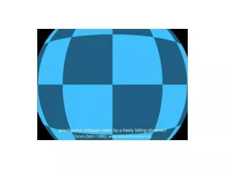
10. Free Falling Frames • Orthonormal bases are parallel transported, so This allows to construct freely falling frames. If we have someone falling from infinity radially inwards in the Schwarzschild metric, then Where the first component is the 4-velocity, but you should check for yourself that the other components are parallel transported.

11. The Field Equation • The field equations are central determining the underlying metric from the distribution of energy. The first step in understanding these is to look at tidal forces. Newton gives If we consider two nearby particles separated by a vector  Taking the leading terms, we get the Newtonian deviation Chapter 21

12. Geodesic Deviation • The separation of two free falling objects gives a measure of the underlying curvature. We need to consider the paths of two nearby geodesics, with a 4-space separation as a function of the proper time along both curves. You must work through the detail (on book webpage) Where the Riemann Curvature tensor is

13. Geodesic Deviation • This is easier to understand in the free falling frame. We need project the deviation vector into the orthonormal frame Remembering what the 4-velocity is in the free falling frame, then Where the Riemann tensor has been projected onto the orthonormal basis.

14. Ge0desic Deviation • In the weak field limit If we assume that our objects fall slowly (non-relativistic) along the geodesics, then the orthonormal and coordinate frame are approximately the same, so We can calculate the Christoffel symbols from the metric and then calculate the components of the Riemann tensor.

15. Geodesic Deviation • Keeping only the lowest order terms, we find In the weak field limit, non-relativistic limit, we recover the result from Newtonian physics. Remember, the Riemann tensor is something that describes geometry, but here it is related to something physical, the gravitational potential.

16. Riemann Tensor • We can drop the leading index in the Riemann Tensor Writing this in a local inertial frame, this becomes Leading to some immediate symmetries; Instead of 256 independent components, this tensor really only has 20 (Phew!)

17. Contractions • Contracting the Riemann tensor gives firstly the Ricci tensor Contracting again gives the Ricci scalar We also have the Kretschmann scalar, which is the measure of the underlying curvature If this is not zero, the spacetime is not flat! For the Schwarzschild metric, we have