Drawing Lines
Drawing Lines. The Bresenham Algorithm for drawing lines and filling polygons. Plotting a line-segment. Bresenham published algorithm in 1965 It was originally to be used with a plotter It adapts well to raster “scan conversion” It uses only integer arithmetic operations


Drawing Lines
E N D
Presentation Transcript
Drawing Lines The Bresenham Algorithm for drawing lines and filling polygons
Plotting a line-segment • Bresenham published algorithm in 1965 • It was originally to be used with a plotter • It adapts well to raster “scan conversion” • It uses only integer arithmetic operations • It is an “iterative” algorithm: each step is based on results from the previous step • The sign of an “error term” governs the choice among two alternative actions
Scan conversion The actual line is comprised of points drawn from a continuum, but it must be “approximated” using pixels from a discrete grid.
The various cases • Horizontal or vertical lines are easy cases • Lines that have slope 1 or -1 are easy, too • Symmetries leave us one remaining case: 0 < slope < 1 • As x-coodinate is incremented, there are just two possibilities for the y-coordinate: (1) y-coordinate is increased by one; or (2) y-coordinate remains unchanged
0 < slope < 1 Y-axis X-axis y increases by 1 y does not change
Integer endpoints ΔY = Y1 – Y0 ΔX = X1 – X0 (X1,Y1) 0 < ΔY < ΔX ΔY (X0,Y0) ΔX slope = ΔY/ΔX
Which point is closer? y = mx + b A yi -1+1 yi -1 B ideal line xi xi -1 error(A) = (yi -1 + 1) – y* error(B) = y* - (yi -1)
The Decision Variable • Choose B if and only if error(B)<error(A) • Or equivalently: error(B) – error(A) < 0 • Formula: error(B) – error(A) = 2m(xi – x0) + 2(y0 – yi -1) -1 • Remember: m = Δy/Δx (slope of line) • Multiply through by Δx (to avoid fractions) • Let di = Δx( error(B) – error(A) ) • Rule is: choose B if and only if di < 0
Computing di+1 from di • di+1 = 2(Δy)(xi+1 – x0) +2(Δx)(y0 – yi) – Δx • di = 2(Δy)(xi – x0) + 2(Δx)(y0 – yi-1) – Δx • The difference can be expressed as: • di+1 = di + 2(Δy)(xi+1 – xi) – 2(Δy)(yi – yi-1) • Recognize that xi+1 – xi = 1 at every step • And also: yi – yi-1 will be either 0 or 1 (depending on the sign of the previous d)
How does algorithm start? • At the outset we start from point (x0,y0) • Thus, at step i =1, our formula for di is: d1 = 2(Δy) - Δx • And, at each step thereafter: if ( d i < 0 ) { di+1 = di + 2(Δy); yi+1 = yi; } else { di+1 = di + 2(Δy-Δx); yi+1 = yi + 1; } xi+1 = xi + 1;
‘bresdemo.cpp’ • The example-program is on class website: http://nexus.cs.usfca.edu/~cruse/cs686/ • It draws line-segments with various slopes • The Michener algorithm (for a circle-fill) is also included, for comparative purposes • Extreme slopes (close to zero or infinity) are not displayed in this demo program • They can be added by you as an exercise
Filling a triangle or polygon • The Bresenham’s method can be adapted • But an efficient data-structure is needed • All the sides need to be handled together • We let the y-coordinate steadily increment • For sides which are “nearly horizontal” the x-coordinates can change by more than 1
Bucket-Sort Y 0 XLO XHI 1 2 8 8 3 7 9 4 6 10 5 5 11 6 7 12 7 9 13 8 11 14 10 13 15 11 15 16 12 17 17 13
Legacy Software • We have a polygon-fill demo: ‘polyfill.cpp’ • You can find it now on our class website • But it was written in 1997 for MS-DOS • We’d like to run it on our Linux system • But it will need a number of modifications • This is our first programming assignment: to “adapt” this obsolete application so it can execute on a contemporary platform
What are some issues? • GNU compiler enforces stricter standards • Sizes of some data-types are now larger • Physical VRAM now must be “mapped” • I/O instructions now require permissions • Real-Mode addresses must be converted • Not all the header-files are still supported • Interface to CPU registers is a bit different
Converting addresses • TURBO-C++ allowed use of ‘far’ pointers • Use a macro to create a pointer to VRAM: • uchar *vram = MK_FP( 0xA000, 0x0000 ); • Real-mode address has two components: (16-bit segment and 16-bit offset) • For Linux we convert to a 32-bit address: uchar *vram = (uchar*)0x000A0000; • Formula: address = 16*segment + offset
Hardware Issues? • Pentium CPUs are “backward compatible” • BIOS firmware can use Virtual-8086 mode • SVGA still supports older graphics modes • The keyboard’s mechanism is unchanged • Feasibility test: if we will “boot” MS-DOS, we can easily run the ‘polyfill’ application • So it’s just a software problem to give our MS-DOS program a new life under Linux!