Channel Routing
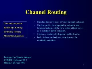
Channel Routing. Simulate the movement of water through a channel Used to predict the magnitudes, volumes, and temporal patterns of the flow (often a flood wave) as it translates down a channel. 2 types of routing : hydrologic and hydraulic.

Channel Routing
E N D
Presentation Transcript
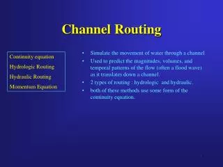
Channel Routing • Simulate the movement of water through a channel • Used to predict the magnitudes, volumes, and temporal patterns of the flow (often a flood wave) as it translates down a channel. • 2 types of routing : hydrologic and hydraulic. • both of these methods use some form of the continuity equation. Continuity equation Hydrologic Routing Hydraulic Routing Momentum Equation
Continuity Equation Continuity equation Hydrologic Routing • The change in storage (dS) equals the difference between inflow (I) and outflow (O) or : • For open channel flow, the continuity equation is also often written as : A = the cross-sectional area, Q = channel flow, and q = lateral inflow
Hydrologic Routing Continuity equation Hydrologic Routing • Methods combine the continuity equation with some relationship between storage, outflow, and possibly inflow. • These relationships are usually assumed, empirical, or analytical in nature. • An of example of such a relationship might be a stage-discharge relationship.
Routing Methods • Kinematic Wave • Muskingum • Muskingum-Cunge • Dynamic Kinematic Wave Muskingum Muskingum-Cunge Dynamic Modeling Notes
MuskingumMethod Sp = K O PrismStorage Sw = K(I - O)X WedgeStorage S = K[XI + (1-X)O] Combined Wedge Prism
Muskingum,cont... Substitute storage equation, S into the “S” in the continuity equation yields : S = K[XI + (1-X)O] O2 = C0 I2 + C1 I1 + C2 O1
Muskingum Notes : • The method assumes a single stage-discharge relationship. • In other words, for any given discharge, Q, there can be only one stage height. • This assumption may not be entirely valid for certain flow situations. • For instance, the friction slope on the rising side of a hydrograph for a given flow, Q, may be quite different than for the recession side of the hydrograph for the same given flow, Q. • This causes an effect known as hysteresis, which can introduce errors into the storage assumptions of this method.
Estimating K • K is estimated to be the travel time through the reach. • This may pose somewhat of a difficulty, as the travel time will obviously change with flow. • The question may arise as to whether the travel time should be estimated using the average flow, the peak flow, or some other flow. • The travel time may be estimated using the kinematic travel time or a travel time based on Manning's equation.
Estimating X • The value of X must be between 0.0 and 0.5. • The parameter X may be thought of as a weighting coefficient for inflow and outflow. • As inflow becomes less important, the value of X decreases. • The lower limit of X is 0.0 and this would be indicative of a situation where inflow, I, has little or no effect on the storage. • A reservoir is an example of this situation and it should be noted that attenuation would be the dominant process compared to translation. • Values of X = 0.2 to 0.3 are the most common for natural streams; however, values of 0.4 to 0.5 may be calibrated for streams with little or no flood plains or storage effects. • A value of X = 0.5 would represent equal weighting between inflow and outflow and would produce translation with little or no attenuation.
More Notes - Muskingum • The Handbook of Hydrology (Maidment, 1992) includes additional cautions or limitations in the Muskingum method. • The method may produce negative flows in the initial portion of the hydrograph. • Additionally, it is recommended that the method be limited to moderate to slow rising hydrographs being routed through mild to steep sloping channels. • The method is not applicable to steeply rising hydrographs such as dam breaks. • Finally, this method also neglects variable backwater effects such as downstream dams, constrictions, bridges, and tidal influences.
Muskingum Example Problem • A portion of the inflow hydrograph to a reach of channel is given below. If the travel time is K=1 unit and the weighting factor is X=0.30, then find the outflow from the reach for the period shown below:
Muskingum Example Problem • The first step is to determine the coefficients in this problem. • The calculations for each of the coefficients is given below: C0= - ((1*0.30) - (0.5*1)) / ((1-(1*0.30) + (0.5*1)) = 0.167 C1= ((1*0.30) + (0.5*1)) / ((1-(1*0.30) + (0.5*1)) = 0.667
Muskingum Example Problem C2= (1- (1*0.30) - (0.5*1)) / ((1-(1*0.30) + (0.5*1)) = 0.167 • Therefore the coefficients in this problem are: • C0 = 0.167 • C1 = 0.667 • C2 = 0.167
Muskingum Example Problem • The three columns now can be calculated. • C0I2 = 0.167 * 5 = 0.835 • C1I1 = 0.667 * 3 = 2.00 • C2O1 = 0.167 * 3 = 0.501
Muskingum Example Problem • Next the three columns are added to determine the outflow at time equal 1 hour. • 0.835 + 2.00 + 0.501 = 3.34
Muskingum Example Problem • This can be repeated until the table is complete and the outflow at each time step is known.