The Normal Distribution
The Normal Distribution. Many thanks to the authors of IB Mathematical Studies Standard Level: For the IB diploma (International Baccalaureate) by Peter Blythe, Jim Fensom , Jane Forrest and Paula Waldman De Tokman (26 Jul 2012).

The Normal Distribution
E N D
Presentation Transcript
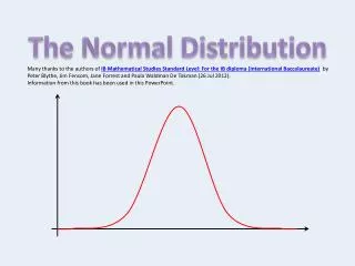
The Normal Distribution Many thanks to the authors of IB Mathematical Studies Standard Level: For the IB diploma (International Baccalaureate) by Peter Blythe, Jim Fensom, Jane Forrest and Paula Waldman De Tokman (26 Jul 2012). Information from this book has been used in this PowerPoint.
The properties of a normal distribution: • It is a bell-shaped curve. • It is symmetrical about the mean, μ. (The mean, the mode and the median all have the same value). • The x-axis is an asymptote to the curve. • The total area under the curve is 1(or 100%). • 50% of the area is to the left of the mean,and 50% to the right. • Approximately 68% of the area is within 1 standard deviation, σ, of the mean. • Approximately 95% of the area is within 2standard deviations of the mean. • Approximately 99% of the area is within 3standard deviations of the mean • The expected value is found by multiplying the number in the sample by the probability.
The properties of a normal distribution: • It is a bell-shaped curve. • It is symmetrical about the mean, μ. (The mean, the mode and the median all have the same value). • The x-axis is an asymptote to the curve. • The total area under the curve is 1 (or 100%). • 50% of the area is to the left of the mean, and 50% to the right. μ
The properties of a normal distribution: • It is a bell-shaped curve. • It is symmetrical about the mean, μ. (The mean, the mode and the median all have the same value). • The x-axis is an asymptote to the curve. • The total area under the curve is 1 (or 100%). • 50% of the area is to the left of the mean, and 50% to the right. 50% 50% μ
The properties of a normal distribution: • It is a bell-shaped curve. • It is symmetrical about the mean, μ. (The mean, the mode and the median all have the same value). • The x-axis is an asymptote to the curve. • The total area under the curve is 1 (or 100%). • 50% of the area is to the left of the mean, and 50% to the right. • Approximately 68% of the area is within 1 standard deviation, σ, of the mean. 68% σ σ μ - σ μ μ + σ
The properties of a normal distribution: • It is a bell-shaped curve. • It is symmetrical about the mean, μ. (The mean, the mode and the median all have the same value). • The x-axis is an asymptote to the curve. • The total area under the curve is 1 (or 100%). • 50% of the area is to the left of the mean, and 50% to the right. • Approximately 68% of the area is within 1 standard deviation, σ, of the mean. • Approximately 95% of the area is within 2 standard deviations of the mean. 95% σ σ σ σ μ -2σ μ - σ μ μ + σ μ +2σ
The properties of a normal distribution: • It is a bell-shaped curve. • It is symmetrical about the mean, μ. (The mean, the mode and the median all have the same value). • The x-axis is an asymptote to the curve. • The total area under the curve is 1 (or 100%). • 50% of the area is to the left of the mean, and 50% to the right. • Approximately 68% of the area is within 1 standard deviation, σ, of the mean. • Approximately 95% of the area is within 2 standard deviations of the mean. • Approximately 99% of the area is within 3 standard deviations of the mean. 99% σ σ σ σ σ σ μ -3σ μ -2σ μ - σ μ μ + σ μ +2σ μ +3σ
Example 1 The waiting times for a elevator are normally distributed with a mean of 1.5 minutes and a standard distribution of 20 seconds. Sketch a normal distribution diagram to illustrate this information, indicating clearly the mean and the times within one, two and three standard deviations of the mean. Find the probability that a person waits longer than 2 minutes 10 seconds for the elevator. Find the probability that a person waits less than 1 minute 10 seconds for the elevator. 200 people are observed and the length of time they wait for an elevator is noted. Calculate the number of people expected to wait less than 50 seconds for the elevator.
Example 1 The waiting times for a elevator are normally distributed with a mean of 1.5 minutes and a standard distribution of 20 seconds. Sketch a normal distribution diagram to illustrate this information, indicating clearly the mean and the times within one, two and three standard deviations of the mean. 1.5 minutes = 90 seconds μ = mean = 90 seconds σ = standard deviation = 20 seconds μ μ -3σ μ -2σ μ - σ μ + σ μ +2σ μ +3σ
Example 1 The waiting times for a elevator are normally distributed with a mean of 1.5 minutes and a standard distribution of 20 seconds. Sketch a normal distribution diagram to illustrate this information, indicating clearly the mean and the times within one, two and three standard deviations of the mean. Find the probability that a person waits longer than 2 minutes 10 seconds for the elevator. 2 minutes 10 seconds = 130 seconds 2.5% or 0.025 Using symmetry about μ, and the fact that approximately 95% of the area is within 2standard deviations of the mean, the two shaded areas together = 5%. So the probability of waiting longer than 2 mins 10 secs is 2.5%, or 0.025. μ μ -3σ μ -2σ μ - σ μ + σ μ +2σ μ +3σ
Example 1 • The waiting times for a elevator are normally distributed with a mean of 1.5 minutes and a standard distribution of 20 seconds. • Sketch a normal distribution diagram to illustrate this information, indicating clearly the mean and the times within one, two and three standard deviations of the mean. • Find the probability that a person waits longer than 2 minutes 10 seconds for the elevator. • Find the probability that a person waits less than 1 minute 10 seconds for the elevator. 2.5% or 0.025 1 minutes 10 seconds = 70 seconds 16% or 0.16 Using symmetry about μ, and the fact that approximately 68% of the area is within 2standard deviations of the mean, the two shaded areas together = 32%. μ μ -3σ μ -2σ μ - σ μ + σ μ +2σ μ +3σ
Example 1 • The waiting times for a elevator are normally distributed with a mean of 1.5 minutes and a standard distribution of 20 seconds. • Sketch a normal distribution diagram to illustrate this information, indicating clearly the mean and the times within one, two and three standard deviations of the mean. • Find the probability that a person waits longer than 2 minutes 10 seconds for the elevator. • Find the probability that a person waits less than 1 minute 10 seconds for the elevator. 2.5% or 0.025 16% or 0.16 μ μ -3σ μ -2σ μ - σ μ + σ μ +2σ μ +3σ
Example 1 The waiting times for a elevator are normally distributed with a mean of 1.5 minutes and a standard distribution of 20 seconds. 200 people are observed and the length of time they wait for an elevator is noted. Calculate the number of people expected to wait less than 50 seconds for the elevator. We already know from part b) that the shaded area represents a probability of 2.5% or 0.025, because 95% of the area is within 2standard deviations of the mean. So, the expected number of people is 2.5% of 200. 200 x 0.025 = 5 5 people μ μ -3σ μ -2σ μ - σ μ + σ μ +2σ μ +3σ
Example 2 The heights of 250 twenty-year-old women are normally distributed with a mean of 1.68m and standard deviation of 0.06m. Sketch a normal distribution diagram to illustrate this information, indicating clearly the mean and the heights within one, two and three standard deviations of the mean. Find the probability that a woman has a height between 1.56m and 1.74m. Find the expected number of woman with a height greater than 1.8m.
Example 2 The heights of 250 twenty-year-old women are normally distributed with a mean of 1.68m and standard deviation of 0.06m. Sketch a normal distribution diagram to illustrate this information, indicating clearly the mean and the heights within one, two and three standard deviations of the mean. μ = mean = 1.68m σ = standard deviation = 0.06m μ 1.68 μ -3σ 1.50 μ -2σ 1.56 μ – σ 1.62 μ + σ 1.74 μ +2σ 1.80 μ +3σ 1.86
Example 2 • The heights of 250 twenty-year-old women are normally distributed with a mean of 1.68m and standard deviation of 0.06m. • Sketch a normal distribution diagram to illustrate this information, indicating clearly the mean and the heights within one, two and three standard deviations of the mean. • Find the probability that a woman has a height between 1.56m and 1.74m. 81.5% The area betweenμ– 2σ and μ = 47.5% because 95% of the whole area is within 2standard deviations of the mean. The area betweenμand μ + σ= 34% because 68% of the whole area is within 1standard deviations of the mean. In fact later we will see that if we calculated this more accurately using the GDC, the value would be 81.9% to 3 s.f. Therefore the area μ– 2σ and μ + σ = 47.5% + 34% = 81.5%. μ 1.68 μ -3σ 1.50 μ -2σ 1.56 μ – σ 1.62 μ + σ 1.74 μ +2σ 1.80 μ +3σ 1.86
Example 2 • The heights of 250 twenty-year-old women are normally distributed with a mean of 1.68m and standard deviation of 0.06m. • Sketch a normal distribution diagram to illustrate this information, indicating clearly the mean and the heights within one, two and three standard deviations of the mean. • Find the probability that a woman has a height between 1.56m and 1.74m. • Find the expected number of woman with a height greater than 1.8m. 81.5% 6 people We can see that the shaded area represents a probability of 2.5%, because 95% of the area is within 2standard deviations of the mean. So, the expected number of people is 2.5% of 250. 250 x 0.025 = 6 μ 1.68 μ -3σ 1.50 μ -2σ 1.56 μ – σ 1.62 μ + σ 1.74 μ +2σ 1.80 μ +3σ 1.86
You can use the GDC to calculate values that are not whole multiples of the standard deviation (or of course even if they are!) Packets of coconut milk are advertised to contain 250ml. Akshat tests 75 packets. He finds that the contents are normally distributed with a mean volume of 255ml and a standard deviation of 8 ml. Find the probability that a packet contains more than 250ml. μ 255 First sketch a normal distribution diagram: μ – σ 247 μ + σ 263 Enter the values: Lower Bound, Upper Bound, μ, σin order, with commas between. μ -2σ 239 μ +2σ 271 μ -3σ 231 μ +3σ 279 In this case: 250, 1E99, 255, 8) Or: 250, 500, 255,8) The solution on the calculator is 0.7340145322 So the probability that a packet contains more than 250ml is 0.734 or 73.4% You could just type in a very large/small number (larger/smaller thanμ +/- 3σ )
Example 3 The lifetime of a light bulb is normally distributed with a mean of 2800 hours and a standard deviation of 450 hours. Find the percentage of light bulbs that have a lifetime of less than 1950 hours. Find the percentage of light bulbs that have a lifetime of between 2300 and 3500 hours. Find the percentage of light bulbs that have a lifetime of more than 3800 hours. 2.95% μ 2800 Sketching the normal distribution diagram gives a clear idea of what is happening. μ – σ 2350 μ + σ 3250 Enter the values: Lower Bound, Upper Bound, μ, σin order, with commas between. μ - 2σ 1900 μ + 2σ 3700 μ - 3σ 1450 μ + 3σ 4150 In this case: -1E99, 1950, 2800, 450) Or: 0, 1950, 2800, 450) The solution on the calculator is 0.0294532933 So the percentage of light bulbs that have a lifetime of less than 1950 hours is 2.95% You can see from the sketch that indeed the answer should be a little more than 2.5%, because there would be 2.5% with a lifetime of less than 1900 hours.
Example 3 The lifetime of a light bulb is normally distributed with a mean of 2800 hours and a standard deviation of 450 hours. Find the percentage of light bulbs that have a lifetime of less than 1950 hours. Find the percentage of light bulbs that have a lifetime of between 2300 and 3500 hours. Find the percentage of light bulbs that have a lifetime of more than 3800 hours. 2.95% 80.7% μ 2800 Sketching the normal distribution diagram gives a clear idea of what is happening. μ – σ 2350 μ + σ 3250 Enter the values: Lower Bound, Upper Bound, μ, σin order, with commas between. μ - 2σ 1900 μ + 2σ 3700 μ - 3σ 1450 μ + 3σ 4150 b) In this case: 2300, 3500, 2800, 450) The solution on the calculator is 0.8068327753 So the percentage of light bulbs that have a lifetime of between 2300 and 3500 hours is 80.7%
Example 3 The lifetime of a light bulb is normally distributed with a mean of 2800 hours and a standard deviation of 450 hours. Find the percentage of light bulbs that have a lifetime of less than 1950 hours. Find the percentage of light bulbs that have a lifetime of between 2300 and 3500 hours. Find the percentage of light bulbs that have a lifetime of more than 3800 hours. 2.95% 80.7% μ 2800 1.31% Sketching the normal distribution diagram gives a clear idea of what is happening. μ – σ 2350 μ + σ 3250 Enter the values: Lower Bound, Upper Bound, μ, σin order, with commas between. μ - 2σ 1900 μ + 2σ 3700 μ - 3σ 1450 μ + 3σ 4150 In this case: 3800, 1E99, 2800, 450) Or: 3800, 0, 2800, 450) The solution on the calculator is 0.0131341011 So the percentage of light bulbs that have a lifetime of of more than 3800 hours is 1.31%
Example 3 The lifetime of a light bulb is normally distributed with a mean of 2800 hours and a standard deviation of 450 hours. Find the percentage of light bulbs that have a lifetime of less than 1950 hours. Find the percentage of light bulbs that have a lifetime of between 2300 and 3500 hours. Find the percentage of light bulbs that have a lifetime of more than 3800 hours. 2.95% 80.7% μ 2800 1.31% 120 light bulbs are tested. d) Find the expected number of light bulbs with a lifetime of less than 2000 hours. μ – σ 2350 μ + σ 3250 Enter the values: Lower Bound, Upper Bound, μ, σin order, with commas between. μ - 2σ 1900 μ + 2σ 3700 μ - 3σ 1450 μ + 3σ 4150 d) In this case: -1E99, 2000, 2800, 450) The solution on the calculator is 0.0377201305 So the percentage of light bulbs that have a lifetime of more than 3800 hours is 3.77% 120 x 0.0377 = 4.5264…. So you would expect 4 or 5 light bulbs
Inverse normal calculations Sometimes you are given the percentage area under the curve, i.e. the probability or the proportion, and you are asked to find the value corresponding to it. This is called an inverse normal calculation. Always make a sketch to illustrate the information given. You must always remember to use the area to the left when using your GDC. If you are given the area to the right of the value, you must subtract this from 1 (or 100%) before using your GDC. 5% 95% For example, an area of 5% above a certain value means there is an area of 95% below it.
Example 4 The volume of cartons of milk is normally distributed with a mean of 995ml and a standard deviation of 5ml. It is known that 10% of the cartons have a volume of less than x. Find the value of x. 989ml Sketching the normal distribution diagram gives a clear idea of what is happening. The shaded area represents 10% of the cartons. Enter the percentage given as a decimal, the mean, and the standard deviation, in order, with commas between. In this case: 0.1, 995, 5) The solution on the calculator is 988.5922422 So x = 989ml (to 3 sig. fig.)
Example 5 The weights of pears are normally distributed with a mean of 110g and a standard deviation of 8g. Find the percentage of pears that weigh between 100g and 130g. It is known that 8% of the pears weigh more than m g. Find the value of m. 250 pears are weighed. Calculate the expected number of pears that weigh less than 105g. μ 110 Sketch a diagram. μ = 110g σ = 8g μ – σ 102 μ + σ 118 μ - 2σ 94 μ + 2σ 126 μ - 3σ 86 μ + 3σ 134
Example 5 The weights of pears are normally distributed with a mean of 110g and a standard deviation of 8g. Find the percentage of pears that weigh between 100g and 130g. 88.8% μ 110 Sketch a diagram. μ = 110g σ = 8g μ – σ 102 μ + σ 118 Enter the values: Lower Bound, Upper Bound, μ, σin order, with commas between. μ - 2σ 94 μ + 2σ 126 μ - 3σ 86 μ + 3σ 134 a) In this case: 100, 130, 110, 8) The solution on the calculator is 0.8881404812 So the percentage of pears that weigh between 100g and 130g is 88.8%
Example 5 The weights of pears are normally distributed with a mean of 110g and a standard deviation of 8g. Find the percentage of pears that weigh between 100g and 130g. It is known that 8% of the pears weigh more than m g. Find the value of m. 88.8% 121g μ 110 Sketch a diagram. μ = 110g σ = 8g μ – σ 102 μ + σ 118 Enter the percentage given as a decimal, the mean, and the standard deviation, in order, with commas between. μ - 2σ 94 μ + 2σ 126 μ - 3σ 86 μ + 3σ 134 In this case the 8% of the pears are to the right of m, so 92% are to the left of m. In this case: 0.92, 110, 8) The solution on the calculator is 121.2405725 So m = 121g (to 3 sig. fig.)
Example 5 The weights of pears are normally distributed with a mean of 110g and a standard deviation of 8g. Find the percentage of pears that weigh between 100g and 130g. It is known that 8% of the pears weigh more than m g. Find the value of m. 250 pears are weighed. Calculate the expected number of pears that weigh less than 105g. 88.8% 121g μ 110 Sketch a diagram. μ = 110g σ = 8g μ – σ 102 μ + σ 118 Enter the values: Lower Bound, Upper Bound, μ, σin order, with commas between. μ - 2σ 94 μ + 2σ 126 μ - 3σ 86 μ + 3σ 134 a) In this case: -1E99, 105, 110, 8) The solution on the calculator is 0.2659854678 So the percentage of pears that weigh between 100g and 130g is 26.6%.c 250 x 0.266 = 66.5, so the expected number of pears that weigh less than 105g is 66 or 67.