GFDL’s CM2 Climate Models

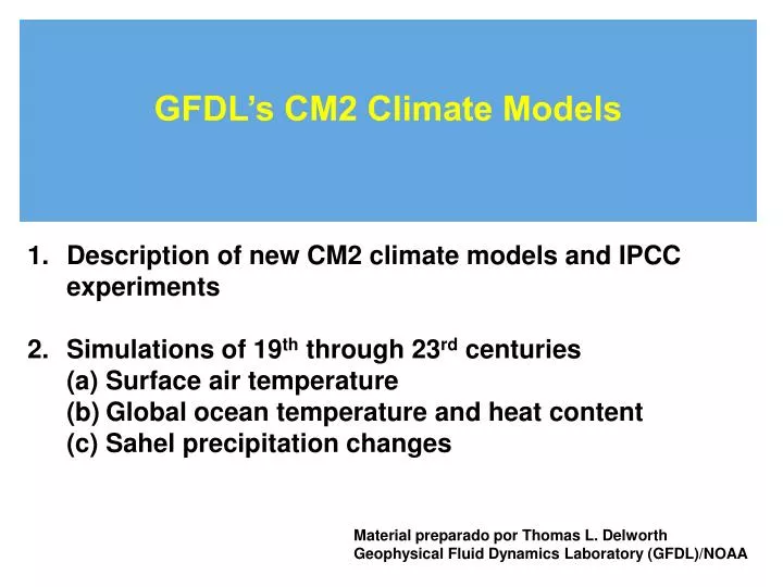
1. GFDL’s CM2 Climate Models • Description of new CM2 climate models and IPCC experiments • Simulations of 19th through 23rd centuries • Surface air temperature • Global ocean temperature and heat content • Sahel precipitation changes Material preparado por Thomas L. Delworth Geophysical Fluid Dynamics Laboratory (GFDL)/NOAA

2. http://www.cdc.noaa.gov/cgi-bin/Composites/printpage.pl Es una pagina interactiva del CDC donde muy rapidamente uno puede calcular composites or regressions de campos atmosfericos u oceanicos. Desde 1958 hasta el presente (campos mensuales). Ncview es una herramienta que les permite ver muy rapidamente campos que tengan en netcdf (mucho mas rapido y en animacion que GRADS) libre. Ferret es una programa para visualizar y hcer todo tipo de graficos ( a la grads pero creo muy superior) libre para linux . Matlab es muy general y muy bueno pero mas restringido que ferret para graficos atmosfericos mu oceanicos.

3. The models used … • New generation of atmosphere, ocean, land and sea ice models developed at GFDL over the last several years. • Atmosphere model referred to as “AM2”. • Coupled model referred to as “CM2.0” and “CM2.1”. A complete suite of experiments has been conducted for the IPCC 2007 report. • AM2 atmosphere (2o horizontal, 24 levels) • MOM4 ocean model, 1o horizontal, 0.3o at Equator, 50 levels) • Sea ice, land models • Detailed descriptions of these models available in GAMDT (2004), Delworth et al. (2005), available on the web at http://data1.gfdl.noaa.gov/nomads/forms/deccen/CM2.X/references Model output available athttp://data1.gfdl.noaa.gov

4. SST Errors (Annual mean Model minus Observations) CM2.0 CM2.1

5. Main algorithmic differences between FV and Bgrid cores horizontal advection of momentum: FV (vorticity) vs centered (u,v) Vertical coordinate and vertical tracer advection: Lagrangian with ppm remapping vs Eulerian ppm Polar filtering “details”

6. Known differences in atmosphere-only (AMIP) mode in fv vs. bgrid Poleward shift of jets and surface westerlies esp. North Atlantic Stronger subtropical easterlies Stronger hydrological cycle (3%) Drier Amazon More eddy activity in polar latitudes

7. 850mb u DJF amip coupled 2.0 2.1

8. Transient eddy v’2 300mb DJF bgrid fv

9. Transient eddy v’2 300mb DJF 2.0 2.1

10. Equatorward drift of jets upon coupling: smaller in CM2.1 than CM2.0; SH shift partly forced from equator, partly locally in SH (P. Kushner – need to check with latest version) Arctic pressures also improve in CM2.1 CM2.1 inherits too strong Pacific winds from AM2_fv: (eddy angular momentum fluxes stronger; and mean tropical rainfall larger than in AM2p13) DJF stationary eddy significantly degraded by coupling over N. America/N.Atlantic (presumably related to redistribution of tropical rain) Somewhat worse in CM2.1 than CM2.0

11. AM2/LM2: comparison to other models Differences in annual mean precipitation from CMAP (Xie-Arkin)

12. Desviacion ClimaticaClimate drift • Coupled models are typically constructed from atmosphere and ocean components that have been independently developed. • Stand-alone atmosphere and ocean components are tightly constrained by observed boundary conditions. • When atmosphere and ocean components are coupled, the resulting climate will often drift away from a realistic state. Material: Anthony Broccolli (Rutgers University

13. Climate Drift in GFDL CM2 Zonal Mean SST Error from CM2_a10o2 [K]

14. Causes of Climate Drift Flux Difference [W m-2]AGCM vs. OGCM CM2_a10o2 SST Error [K]

15. Causes of Climate Drift • Imbalances between atmosphere-ocean heat fluxes simulated by AGCM and OGCM when both are run with observed SSTs. • Climate feedbacks triggered by flux imbalances. (Ex: CM2_a10o2 cooling pattern in midlatitude N.H. → southward shift in westerlies → error in position of western boundary currents)

16. Flux Corrections/Adjustments • One ad hoc approach to reducing climate drift is to adjust for differences in atmospheric and oceanic component fluxes by adding a compensating flux at each grid point. • This method is known as flux correction (Sausen et al. 1986) or flux adjustment (Manabe et al. 1991).

17. Calculating Flux Adjustments • The goal is to determine artificial heat and water fluxes that vary seasonally and spatially but do not depend on the state of the model. • Method 1: GFDL Three-Step • Method 2: Coupled Restore • Method 3: Offline Flux Difference

18. Method 1: GFDL Three-Step • Step 1: Run the AGCM with climatological SSTs, archiving the heat and water fluxes. • Step 2: Run the OGCM with the fluxes from step 1, while simultaneously restoring to observed T and S.

19. Method 1: GFDL Three-Step • Step 1: Run the AGCM with climatological SSTs, archiving the heat and water fluxes. • Step 2: Run the OGCM with the fluxes from step 1, while simultaneously restoring to observed T and S. Restoring terms

20. Method 1: GFDL Three-Step • Step 1: Run the AGCM with climatological SSTs, archiving the heat and water fluxes. • Step 2: Run the OGCM with the fluxes from step 1, while simultaneously restoring to observed T and S. • Step 3: Couple the AGCM and OGCM without restoring, using the archived restoring terms from step 2 as flux adjustments.

21. Flux Adjustment: Pros and Cons Cons • Flux adjustments are nonphysical. • There is no guarantee that coupled model biases are invariant over different climate states. • Flux adjustments could distort climate feedbacks.

22. Flux Adjustment: Pros and Cons Pros • Flux adjustments minimize climate drift that would distort climate feedbacks if left unchecked. • Flux adjustments allow sensitivity experiments to be performed while better models (i.e., those with smaller errors) are under development.

23. Design of Coupled Model Experiments • Equilibrium: The goal is to determine the climate that is in equilibrium with a given set of climate forcings. (Example: What climate state is in equilibrium with twice the preindustrial level of atmospheric CO2?) • Transient: The goal is to investigate the time-dependent response of the climate to a given (often time-dependent) change. (Example: How will the climate change in response to projected increases in CO2 and other human-induced climate forcings?)

24. CM2.1 CM2.0 Minimal climate drift after spinup W m-2 • 200 300 400 500 600 700 800 Model Year

25. (8 member ensemble of1861-2000 experiments)

26. Ensemble simulations of the 20th century • ALL – includes ghgs, strat ozone, anthrop. aerosols, land use, solar,volcanoes • ANTHRO • NATURAL • AEROSOL (anthropogenic aerosols) • WMMGO3 (well mixed ghgs, stratospheric ozone)

27. Knutson et al., submitted

28. OBS SST 77-95 minus 49-66 3-member ensemble mean CM2.0 5-member ensemble mean CM2.1

30. Krakatau ALL FORCINGS NATURAL ANTHRO

31. AEROSOLS (ANTHRO) WMGGO3

32. January Observed Precipitation (mm/month) Data from Univ. of East Anglia, Climatic Research Unit (CRU) July Seasonal migration of Intertropical Convergence Zone (ITCZ)

33. 1950-2000 trends in observed and simulated precipitation (JAS) Simulated Observed (Atmosphere model forced with observed SSTs 1950-2000)

34. Simulated effect of Observed 1950-2000 SST trend on African precipitation GLOBAL SSTs PAC ONLY ATL ONLY INDIAN ONLY

35. 1950-2000 linear trend in precipitation Observed CM2.0 20th century historical run CM2.1 20th century historical run

36. Future perspective 20th century historical runs 1951-2000 CM2.1 CM2.0 A1B scenarios 2001-2050 CM2.1 CM2.0

37. Observations 21st century scenarios Model ensemble mean

38. Summary/Conclusions • Suite of 20th century simulations with new GFDL climate models. Output freely available on the Web. http://data1.gfdl.noaa.gov • 2. Simulated air temperature trends largely consistent with observed trends. • Simulated ocean temperature and heat content changes “consistent” with observations. Strong role for aerosols (natural and anthropogenic) in simulated 19th and 20th century changes. • 4. GFDL models (a) simulated the 20th century Sahel drought as a response to anthropogenic forcing, and (b) project the Sahel drying to continue into the future. This is generally not seen in other coupled models, and is thus highly uncertain.

39. Comparing the climate sensitivity of AM2/LM2 to the new NCAR CAM2 Ensemble of the world’s climate models (IPCC 2001)

40. Low cloud behavior in models run with observed SSTs (1952-1997) Analysis performed by Joel Norris (UCSD)

41. Cubed Sphere Core Lat-Lon Core

42. The C360 (~ 28 km) tropical cyclone-climate model • Dynamics: non-hydrostatic Cubed Sphere FV core • Physics: GFDL AM 2.1 (identical to CM2.1 for IPCC AR4) • “Cold” start (isothermal, dry, wind-less) from 00Z Jan 1, 1980 • Forced with “observed” SST 3-hourly precipitation: 1-31 August 1980

43. Corridas de sensibilidad al incremento de CO2

44. Vientos la componente u en 850hPa

45. Precipitacion

46. Ozono en la baja estratosfera

47. Final notes: • The “cubed sphere” core development is in a mature stage. But the application side of the work has just been started…..the codes that contains the cubed sphere model within GFDL’s atmosphere-ocean-land-ice coupling system were released internally in Aug 2007. • Experimental dynamical seasonal hurricane/typhoon predictions will be made at GFDL (starting FY07-08) at global ¼ (C360) to 1/8 deg (C720) resolutions. • With the non-hydrostatic cubed sphere dynamical core, it is feasible to make global cloud resolving runs at 4~5km resolution with existing massively parallel computers in the US (e.g., DOE/Oak Ridge or NASA Columbia?). The model is fast enough to be used for real-time10-day hurricane predictions – a potential breakthrough for hurricane forecasting

48. FIN