Evaluating Climate Envelope Models for Florida's Endangered Vertebrates: The Role of Extremes
10 likes | 140 Views
This study investigates the performance of Climate Envelope Models (CEMs) for Florida's threatened and endangered vertebrates between 1981 and 2010, assessing whether incorporating extreme climate variables improves model accuracy. Utilizing three metrics—AUC, Cohen's kappa, and True Skill Statistic (TSS)—the results show no significant improvement from including extreme variables, despite higher spatial correlations for certain species. The findings raise questions about the necessity of adding extremes to CEMs, suggesting that their impact may be better assessed at broader scales or across different species.

Evaluating Climate Envelope Models for Florida's Endangered Vertebrates: The Role of Extremes
E N D
Presentation Transcript
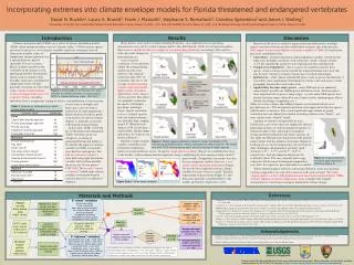
PRISM3monthlytemp./precip. grids (1981- 2010) Incorporating extremes into climate envelope models for Florida threatened and endangered vertebrates • David N. Bucklin1, Laura A. Brandt2, Frank J. Mazzotti1, Stephanie S. Romañach3, Carolina Speroterra1 and James I. Watling1 • 1University of Florida Fort Lauderdale Research and Education Center, Davie, FL, USA; 2U.S. Fish and Wildlife Service, Davie, FL, USA; 3U.S. Geological Survey,Southeast Ecological Science Center, Davie, FL, USA Introduction Results Discussion • Three metrics were used to evaluate model performance - area under the receiver operating characteristic curve (AUC), Cohen’s kappa, and the True Skill Statistic (TSS). For all species together, there were no significant one-way changes in average model performance according to these metrics, with only small changes for Climate envelope models (CEMs) are a subset of species distribution models (SDM) which attempt to define a species’ climate “niche.” CEMs correlate species presence locations to a set of climatic variables, which are commonly derived Because of the lack of conclusive improvement in model metrics and high spatial correlation between models with/without extremes, this study provides little support for universal addition of extreme variables to CEMs. Several factors may have contributed to this: IBTrACS4 tropical cyclone dataset (1900-2010) from mean monthly values of temperature and precipitation over a specified historic period (generally 30 years or more). Mean variables smooth out the variability in the climate record, ignoring potentially deterministic factors such as rainfall events, droughts, hurricanes, and high/low temperature events. Despite generally occurring on a short time scale, extreme weather/climate events can impact many aspects of a species’ biology, including • individual species. • A test of spatial correlation (r) revealed how similar the testing/training models (n=100) were relative to the “default” model run with 100% of occurrence data (n=1). On average, models including extremes had significantly higher spatial correlation (paired t-test, n=16, mean = +0.014, p<0.05). This effect was primarily evident for the species with higher prevalence and larger ranges. Spatial correlation between “default” models with and without extremes was generally high, ranging from 0.87 (Bluetail mole skink) to 0.99 (Lower Keys marsh rabbit). Model output and metrics for 8 species are shown in Figure 2. • MaxEnt’s output includes variable contribution and permutation importance • Correlation - extreme temperature and precipitation variables created for this study were all highly correlated with at least one “mean” climate variable (r > 0.84), limiting the amount of novel information they could provide • Temporal correspondence - due to scarcity of occurrence data for most species, some occurrences from outside the temporal domain were used; this may be more relevant to extreme climate due to its short-term impact • Spatial scale - while climate undoubtedly plays a role in species distributions, it is possibly a more appropriate determinant at courser scales and across a wider geographic domain than used in this study • Applicability for some study species – many T&E species are inherently range-limited, possibly not fulfilling their full abiotic niche. Extremes play a more important role at species’ range edges1; as such, many T&E species have already had their ranges reduced by non-climatic factors (anthropogenic effects, habitat loss/change, competition, etc.). Climate extremes increasing since 1970 individual fitness, morphology, timing of activity, and distribution; certain extreme There was someevidence that adding extremes was beneficial for the most prevalent species - TSS and spatial correlation were improved for the four species with the most occurrences. The overall significant improvement in spatial correlation does not indicate that models including extremes were “better” - just more similar to the “default” model. events (such as droughts and hurricanes) can even lead to extinctions of entire populations.1 Recent historical evidence points to an increase in extreme climate (Figure 1), generally associated with ongoing climate change. In this study, CEMs were built for 16 threatened and endangered (T&E) vertebrate species or subspecies occurring in peninsular Florida and the Keys. To identify the impact of extreme variables in CEMs, two models were built for each species. The first set of models (“means”) were built using eight bioclimatic variables derived from monthly means for the 30-year period 1981-2010.The second, (“means + extremes”) added eight extreme variables to the predictor pool (listed in Materials and Methods diagram). • Figure 1. Percentage of contiguous U.S. area affected by climate extremes as measured by NCDC’s Climate Extreme Index, 1910-20112 • Addition of extremes will probably be most beneficial is cases where there are empirically-derived physiological limits or well-documented responses to climate/weather events, allowing for hypothesis testing and better predictions into future climates. In this study, the Bluetail mole skink showed the greatest improvement with the addition of extremes (Figure 4). Looking just at extreme temperatures, the envelope of daily minimums and maximums are fairly small (between -3.8⁰ – -2.7⁰ C and 36.7⁰– 36.9⁰ C, respectively), with the minimum likely near the ectotherm’s limit. This may currently deter range expansion, but increases in minimum temperatures may allow for expansion, provided habitat is available. • Figure 2. Model spatial predictions (“default” model, threshold at 10% occurrence probability value, metrics (calculated as mean value for 100 model runs with 75/25 training/testing split), and occurrences for eight species • metrics for each model run. Across all species, temperature seasonality (Figure 3a) contributed the most to the models, with maximum diurnal temperature range contributing the most among extremes (and 2nd • Figure 4. Model predictions for the Bluetail mole skink (following Figure 2) • most overall). Temperature seasonality was also the most important variable; however, 1-year return extreme minimum temperature (Figure 3b) was the most important extreme climate variable (but only 4thmost overall). Variables representing tropical storms (Figure 3c) and hurricanes generally contributed little to the models and had low importance scores. c a b While climate changes’ effect on extreme precipitation events are uncertain, extreme temperatures are expected to increase with some certainty.7 For wide-ranging species, or those with populations near known physiological limits, CEMs with the addition of extreme temperatures alone could provide valuable information for conservation managers planning for climate change. • Figure 3a,b,c. Three study variables Materials and Methods References 1 Parmesan, C., T. L. Root, and M.R. Willig. 2000. Impacts of Extreme Weather and Climate on Terrestrial Biota. Bulletin of the American Meteorological Society 81 (3):443-450. 2 Gleason, K. L., J. H. Lawrimore, D. H. Levinson, T. R. Karl, and D. J. Karoly. 2008. A revised US Climate Extremes Index. Journal of Climate21 (10):2124–2137. 3 PRISM Climate Group, Oregon State University. Accessed 2011. 2.5-arcmin (4 km) Monthly climate data. http://prism.oregonstate.edu. 4 Knapp, K. R., M. C. Kruk, D. H. Levinson, H. J. Diamond, and C.J. Neumann. 2010. The International Best Track Archive for Climate Stewardship (IBTrACS): Unifying tropical cyclone best track data. Bulletin of the American Meteorological Society 91:363-376. 5 Nix, H.A. 1986. A biogeographic analysis of Australian elapid snakes. In Atlas of elapid snakes in Australia, ed. R. Longmore: 4-15. 6 Phillips, S.J., R.P. Anderson, and R.E. Schapire. 2006. Maximum Entropy Modeling of Species Geographic Distributions. Ecological Modelling 190 (3–4):231–259. 7 Kharin, V. V., F.W. Zwiers, X. Zhang, and G. C. Hegerl. 2007. Changes in Temperature and Precipitation Extremes in the IPCC Ensemble of Global Coupled Model Simulations. Journal of Climate 20 (8):1419–1444. 8 “mean” variables Annual mean temp. Temp.seasonality Max. temp. of warmest month Min.temp. of coldest month Annual precipitation Precipitation seasonality Precipitation of wettest quarter Precipitation of driest quarter “means” model (“default”); 100% of data (n=1) Monthly tmin, tmax, precip. averages calculated to create 19 bioclimatic variables5 MaxEnt 3.3.3a6 “means” models, with 75/25 training/testing split (n = 100) MaxEnt 3.3.3a6 6 extreme temp./precip. variables calculated; interpolated using ordinary kriging 16 species’ presencedatasets (Table 1; from literature/online sources) NCDC daily temp./precip. (1981-2010, 100 stations) “means+extremes” (“default”)with 100% of data(n=1) Acknowledgements 8 most important variables selected “means+extremes” models created with all 16 variables MaxEnt 3.3.3a6 8 “extreme” variables Daily extreme max. temp., 1-year return • Daily extreme min. temp., 1-year return Mean annual max. diurnal temp. range • 1-day precip. event, 1-year return • 7-day precip. event, 1-year return Mean annual # of precip. days >=50 mm • Tropical storms (total # within 40km) • Hurricanes (total # within 40km) Funding was provided by the U.S. Fish and Wildlife Service, National Park Service Everglades and Dry Tortugas National Park, through the South Florida and Caribbean Cooperative Ecosystem Studies Unit and U.S. Geological Survey (Greater Everglades Priority Ecosystems Science). Thanks to Melissa Griffin at the Florida Climate Center for providing climate data for Florida stations. “means+extremes” models, with 75/25 training/testing split (n = 100) • Tropical storm and hurricane variables created All variables were resampled to a 4-km resolution and clipped to the state of Florida boundary prior to modeling. A “one-year return” indicates a daily extreme value/event that happens once a year, on average. Tropical storms and hurricanes are defined as storms with winds greater than 34 and 64 knots, respectively. Please contact david.bucklin@gmail.comfor more information on this project. More information on the climate envelope modeling project at UF-FLREC can be found at http://crocdoc.ifas.ufl.edu/projects/climateenvelopemodeling/.