Download
1 / 43
500 likes | 690 Views
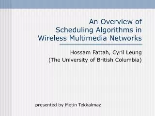
An Overview of Scheduling Algorithms in Wireless Multimedia Networks. 李孝治 Hsiao-Chih George Lee http://www.en.oit.edu.tw/lee mailto://lee@en.oit.edu.tw. Abstract.

E N D
An Overview of Scheduling Algorithms in Wireless Multimedia Networks 李孝治 Hsiao-Chih George Lee http://www.en.oit.edu.tw/lee mailto://lee@en.oit.edu.tw
Abstract • Scheduling algorithms are important components in the provision of guaranteed quality of service parameters such as delay, delay jitter, packet loss rate, or throughput. • The design of scheduling algorithms for mobile communication networks is especially challenging given highly variable link error ratesand capacities, and the changing mobile station connectivity. • This article provides • a survey of scheduling techniques for several types of wireless networks. • Scheduling algorithms for TDMA, CDMA, and Multihop networks.
Introduction • QoS requirements for different service classes:
Wireless Network Scheduler Challenges • Characteristics of wireless links • Subject to time- and location-dependentsignal attenuation, fading, interference, and noise that result in bursy errors and time-varying channel capacities. • Wireless channel model • Discrete-time Markov chain with two states: error-free (“good”) or error-prone (“bad”) • A packet is successfully received if and only if the link stays in the good state throughout the packet transmission time.
Information needed to make scheduling decisions • Number of sessions • Session reserved rates • Link states • Statuses of session queues • Information availability • For the down-link: • The scheduler is located at the base station (BS) • This information is easily obtianed • For the up-link: • Some means must be provided to collect queue status information and to inform mobile stations (MSs) of their transmission times.
To maximize MS battery life • To transmit/receive in contiguous time slots and then go into a sleep mode rather than to rapidly switch among transmit, receive and sleep modes. • Handoffs • Following a handoff, any packets for S that are queued at previous cell C1’s BS will be forward to current cell C2’s BS • For timestamp-based scheduling • Timestamp update • Fairness gap: low timestamp extra service
In CDMA network, • the total interference at an MS must be small enough to ensure an adequate signal-to-interference ration (SIR) for each session, thereby enabling its target bit error rate (BER) to be met. • The scheduler must ensure that the number of simultaneous transmissions in the network is not so high as to result in excessive interference. • In multihop networks • No BSs • Rapidly changing topology • Routing
Scheduler Components and Properties • Components (1) An error-free service model (2) A lead/lag counter • Whether the session is leading, in sync with, or lagging its error-free model and by how much (3) A compensation model for each session • A lagging session is compensated at the expense of leading sessions
(4) Separateslot queues and sessionqueues for each session • When a packet arrives, it is timestamped and placed in the packet queue; • A slot with the sametimestamp value is added to the slot queue. • If the HOL (Head of line) packet for a session is dropped due either to excessive delay (delay-sensitive) or an excessive number of retransmissions (error-sensitive), the precedence of the session for accessing the channel is maintained by the slot queue. (5) A means for monitoring and predicting the channel state for every backlogged session.
Features • Efficient link utilization: • Delay bound: • Fairness: • Throughput: • Implementation complexity: • Graceful service degradation: • Isolation: • Energy consumption: • Delay/bandwidth decoupling: • Scalability:
Scheduler Classification • Work-conserving • The scheduler is never idle if there is a packet awaiting transmission. • Generalized Processor Sharing (GPS)Weighed Fair Queueing (WFQ)Virtual Clock (VC)Weighted Round Robin (WRR)Self-Clocked Fair Queueing (SCFQ) Deficit Round Robin (DRR)
Non-work-conserving • The scheduler may be idle even if there is a backlogged packet in the system because it may be expecting another higher-priority packet to arrive. • Hierarchical Round-Robin (HRR) Stop-and-Go Queuing (SGQ)Jitter-Earliest-Due-Date (Jitter-EDD) Higheraveragepacket delays than work-conserving May be used in application where jitter is more important thandelay
Timestamped • Incoming packets are timestamped before being placed in their respective session queues. • The HOL packets are then sorted in increasing order of their timestamps, and the packet with the lowest timestamp value is selected for transmission. • Better QoS guarantees • Round-robin • No timestamps • Easily implemented
Sorted-priority • Each session has a different priority level • Packets are chosen for transmission according to their session priority • VC, WFQ, Jitter-EDD • Frame-based • Time is divided into frames of fixed or variablesize • Each session reserves a portion of the frame for transmission • Non-work-conserving • HRR, SGQ – fixed-size frames • WRR, DRR, FFQ (Frame-based Fair Queueing) – variable-size frames
Generalized Processor Sharing-Based Scheduling • GPS • An ideal fluid flow model that services all sessions simultaneously • Work-conserving • PGPS (Packet GPS) • To emulate GPS by serving packets in increasing order of their timestamps
Scheduling Algorithms for Wireless TDMA Networks • Network Model • One BS and a number of MSs. • Scheduling is implemented at the BS, which can communicate with all MSs; • Direct MS-to-MS communication is not possible. • Channel errors. • Knowledge of the channel state and packet queue status for all sessions is available at the BS.
Channel State Dependent Packet Scheduling (CSDPS) • To avoid bursty errors at the link layer • Allow the use of differentservice disciplines • RR • Longest Queue First (LQF) • Earliest Timestamp First (ETF) • Channel state for each session is monitored. • If the channel for a session is in a bad state, the transmission of this packet is deferred. • No lead and lag • No compensation
Idealized Wireless Fair Queueing (IWFQ) • Realization of PGPS with a compensation • Error-free network model: WF2Q • Each session has a service tag that is equal to the virtual finish time of its HOL packet. • Lagging sessions will have the lowestservice tag values • Bound on the lead and lag session • Not graceful: lagging session capture the channel until it has been compensated for all its lag
Channel-Condition-Independent Fair Queueing(CIFQ) • Use of Start-time Fair Queueing (SFQ) • Scheduling is based on the start time • Each session has a lead and lag counter • Graceful service: • A leading session retainsa fraction [0, 1] of its service • No lead/lag counter bound is needed
Server-Based Fairness Approach (SBFA) • A portion of the outgoing bandwidth is reserved for a hypothetical session called a Long-Term Fairness Server (LTFS). • The LTFS is used to compensate lagging sessions. • When a session is selected for transmission, it is not allowed to transmit if it has a badchannel, a slot for this session is created and queued into the LTFS session. • No lead/lag counter • The compensation rate depends on the reserved bandwidth for LTFS.
Wireless Fair Service (WFS) • Timestamp: • Sessions are selected for transmission in increasing order of their service tag values provided that the virtual start time of the HOL packet is less thanv(t) + where is a look-ahead parameter that determines the schedulable interval. • If = and Ri =i, the error-free service is WFQ. • If = 0and Ri =i, the error-free service is WF2Q. • Lead/lag counter
Scheduling in CDMA Networks • Advantages of CDMA over TDMA and FDMA • higher (soft) system capacity • soft handoff • simple frequency planning • inherent frequency diversity against multipath fading • Voice activity factor and antenna sectorization are readily exploited using CDMA. • Drawback • an accuratepower control mechanism is required.
Properties of CDMA • The soft capacity feature of CDMA allows a new session to be established provided that the for all transmitting sessions can be maintained above their target levelsa certain percentage of the time [11]. • The packets sent from a number of MSs can be successfully receivedsimultaneously at the BS, provided an adequatepower control scheme is used.
Packet-By-Packet GPS (PGPS) • A residualpower index that is not utilized. • To find one or more additional (non-HOL packets) packets which can be transmitted.
Scheduled CDMA (SCDMA) • A hybrid CDMA/TDMA scheduler in which the BS schedules transmissions of the MSs as shown in Fig. 2. • A fixed-size unit called capsule which can accommodate one or more packets. • All MSs in a cell have the samecapsule size. • Assume a time-slotted operation • For uplink scheduling (1)A capsule transmission request (CTR) is sent to BS by an MS (2) The BS sorts the CTRs according to their priority level or delay tolerance and places them in a global queue. (3) The BS sends transmission permission to the selected MS to inform of their capsule transmission times and power levels
Dynamic Resource Scheduling (DRS) • Centralized and adaptive • MSs send their requests to the BS • The BS classifies them according the traffic characteristics of the requested service and places them in two separate queues: guaranteed queue (CBR, VBR, minimum-rate ABR) and best-effort queue(UBRand excess ABR) • Neither DRS and SCDMA provide guaranteed delay bound
Wireless Multimedia Access Control Protocol with BER Scheduling (WISPER) • Packets are transmitted within frames of length T in both uplink and downlink, • The uplinkrequestslot is used by an MS to place transmission requests. • The downlinkcontrol slot is used by the BS to grant transmission permissions. • Traffic classes with a different BER requirement • The selected packets are grouped into the N slots according to the following order: • Same BER、stricker BER、looser BER
Scheduling in Multihop Networks • Network Model • Base stations are not available • Single-hop networks • Each MS can communicate directly with all other MSs • multi-hop networkMobile Ad-hoc Networks (MANETs) • Not all MSs can communicate directly with each other. • MSs, acting as relays, are then needed to forward packets to their final destinations.
Scheduling in Multihop Networks • Base stations are not available • Single-hop networks • Each MS can communicate directly with all other MSs • multi-hop networkMobile Ad-hoc Networks (MANETs) • Not all MSs can communicate directly with each other. • MSs, acting as relays, are then needed to forward packets to their final destinations.
Network Model • Time is assumed to be divided into slots, each of duration equal to one maximum-length packettransmission timeplus the maximum propagation time between any two MSs. • Omni-directional antenna • Noise-free an unsuccessful reception is due only to collisions. • Half-duplexan MS can transmit or receive, but cannot do bothat the same time.
F F C D C D G • Conflict Types in Multihop Scheduling • Two types of conflicts • A primary conflictoccurs when two or more MSs simultaneously transmit to a common destination node(e.g., nodes C D & F D). • A secondary conflictoccurs when an MS receiving a transmission intended for it is interfered with by another transmission not intended for it; (e.g., C D & F G) Different spreading code a secondary conflict can be tolerated
Scheduler Properties • Topology transparency: • The scheduler should work efficiently regardless of how frequently and unpredictably the topology changes. • A topology independent algorithm reduces the burden of having to recompute and reassign time slots. • Low connectivity information requirement: • Some algorithms need global network connectivity information while others require only local(e.g., one- or two-hop) connectivity information. • Scheduler Examples • Node activationscheduler • Link activationscheduler
(1)Node activationscheduler • selects nodes for transmission to ensure that a packet transmission from any node will be received correctly by all its neighbors. • Each MS has network connectivity information within a two-hop radius. • Each MS i is allocated the ith time slot in a frame • MSs more than two hops away from the MS i are also eligible to transmit during slot i. • Some pre-established rule is used to select an eligible MS to transmit in slot i. • The selected MS sends a broadcast message to inform other MSs that it is using slot i. • It does not ensure fair slot allocations among all MSs and is nottopology-transparent.
Scheduler Examples (1)Node activationscheduler • selects nodes for transmission to ensure that a packet transmission from any node will be received correctly by all its neighbors. • Each MS has network connectivity information within a two-hop radius. • Each MS i is allocated the ith time slot in a frame • MSs more than two hops away from the MS i are also eligible to transmit during slot i. • Some pre-established rule is used to select an eligible MS to transmit in slot i. • The selected MS sends a broadcast message to inform other MSs that it is using slot i. • It does not ensure fair slot allocations among all MSs and is nottopology-transparent.
(2) Link activationscheduler • selects nodes for transmission to only guarantee that the destination node receives the packet successfully. • MS i uses a time slot assignment function(TSAF) to locate its transmission slots in a frame. • The TSAF, fi(x), is a polynomial of degree k with coefficients in {0, 1, …, p –1} where p is a prime number. • Polynomial evaluation is done using mod parithmetic. • Each frame is divided into p subframes, each consisting of p slots. • MS i is assigned one slot in each subframe as follows: in subframe j, j = 0, 1, …, p– 1, the assigned slot number is given by fi(j). • A collisionoccurs between MS i and MS l in subframe j if fi(j) = fl(j).
Conclusion • Much work remains to be done in the design and performance evaluation of wireless schedulers, especially forCDMA and multihopnetworks.