Download
1 / 61
790 likes | 1.12k Views
Online Algorithms. Introduction. An offline algorithm has a full information in advance so it can compute the optimal strategy to maximize its profit (minimize its costs).

E N D
Introduction An offline algorithm has a full information in advance so it can compute the optimal strategy to maximize its profit (minimize its costs). An online algorithm is a strategy which at each point in time decides what to do based only on past information and with no (or inexact) knowledge about the future.
Typically when we solve a problem we assume that we know all the data a priori. However, in many situations the input is only presented to us as we proceed. Definition: The competitive-ratio of algorithm A is CA if for any n > N0 and for any sequence Rn, where c is independent of n.
s £ a × s C ( ) C ( ) A OPT on C is the cost of the online strategy A on Definition 1: An onlinealgorithmAon is a-competitive if for all input sequences s, where: COPT is the cost of the optimal offline algorithm In order to evaluate the online strategy we will compare its performance with that of the best offline algorithm. This is also called competitive analysis.
s £ a × s + C ( ) C ( ) c A OPT on C is the cost of the online strategy A on Definition 2: An online algorithmAon is a-competitive if for all input sequences s, where:COPT is the cost of the optimal offline algorithm c is some constant independent of s
Definition Input: linked list a sequence I of requested accesses where . The cost of accessing is the location of the item in the list counted from the front. Given I (online), our objective is to minimize the cost of accessing the items in the list The List Accessing Problem
While processing the accesses we can modify the list in two ways: free transpositions: after an access, the requested item may be moved at no cost closer to the front of the list. paid transpositions: at any time we can swap two adjacent list items at a cost of 1.
Deterministic Online Algorithms Move-To-Front (MTF) Move the requested item to the front of the list. Transpose (TRANS) Exchange the requested item with the immediately preceding item in the list Frequency-Count (FC) Maintain a frequency count for each item in the list. Items are stored in non-decreasing order of accesses. After item is accessed its frequency counter is updated and item moved forward (if necessary) to maintain list order.
We will prove the following two facts: Theorem 1: The Move-To-Front algorithm is 2-competitive. Theorem 2: Let A be a deterministic online algorithm for the List Accessing Problem. If A is c-competitive, then . Pay attention to the fact that in theorem 2 we prove a lower bound to the competitiveness.
Proof 1: Definitions: The potential function F: For any F(t) = The number of inversions in Move-To- Front’s list with respect to OPT’s list, after is served. An inversionis a pair x,y of items such that x occurs before y in Move-To-Front’s list and after y in OPT’s list.
Move-To-Front and OPT start with the same list, so the initial potential is 0. We will show that for any t then and because the theorem follows. The amortized cost incurred by Move-To-Front on is defined as
We will show inequality (*) For an arbitrary t. Let: x = the item requested by . k = number of items before x in MTF’s and OPT’s list l = number of items before x in MTF’s list but follow x in OPT’s list. When MTF serve and moves x to the front of the list, l inversions are destroyed and at most k new inversions are created. Thus
Proof 2: Consider a list of l items. n requests in I. We construct a “bad” request sequence for A with cost Let OPT be the optimum static offline algorithm. OPT first sorts the items in the list in order of nonincreasing request frequencies and then serves I without making any exchanges. If the list is sorted by request frequencies, the worst case is that all frequencies are n/l (then we didn’t gain anything from sorting). Thus accesses costs:
We can take instead of OPT the static offline algorithm because we prove a lower bound. Each request is made to the item that is stored at the last position in A’s list. n requests, each will cause cost l, lead us to the cost nl. If the frequencies are not equal the cost will be lower, because then we’ll put the more frequent items closer to the beginning, causing more cheap accesses and less expensive accesses.
Rearranging the list cost at most l(l-1)/2. Then the requests in I can be served at a cost of at most n(l+1)/2. Thus The theorem follows because the competitive ratio must hold for all list lengths.
Randomization Algorithm Bit Each item in the list maintains a bit that is complemented whenever the item is accessed. If an access cause a bit to change to 1, then the requested item is moved to the front of the list. The bits are initialized independently and uniformly at random. Theorems: 1. The Bit algorithm is 1.75-competitive against any oblivious adversary. 2. Let A be a randomized online algorithm for the List Accessing Problem. If A is c-competitive against any oblivious adversary, then .
The k-Server Problem Motivation: There are k servers for your drink requests. They come sequentially, and the response is quick (before the next request is up). Special cases of the k-server problem • Paging • The k-server problem with a uniform distance metric. • Two-headed Disk • k servers are the 2 heads
Paging • The paging problem is a special case of the k-server problem, in which the k servers are the k slots of the fast memory, V is the set of pages and d(u,v)=1 for uv. In other words, paging is just the k-server problem but with a uniform distance metric. • Two-headed Disk • You have a disk with concentric tracks. Two disk-heads can be moved linearly from track to track. The two heads are never moved to the same location and need never cross. The metric is the sum of the linear distances the two heads have to move to service all disk’s I/O requests. Note that the two heads move exclusively on the line that is half the circumference and the disk spins to give access to the full area.
A metric space is a set of points V along with a distance function Definition 1: The k-Server Problem s.t.
Sometimes it is convenient to think of a finite metric space over n points as the complete weighted graph over n vertices with weights corresponding to distance between the corresponding points. Similarly, given a weighted (not necessarily complete) graph, we can associate a metric space with it by letting the distance between any pair of points to be the (weighted) length of the shortest path between them in the graph.
The input is a metric space V, a set of k “servers” located at points in V, and a stream of requests 1,2,…, each of which is a point in V. For each request, one at a time, you must move some server from its present location to the requested point. The goal is to minimize the total distance traveled by all servers over the course of the stream of requests. Definition 2: (The k-server problem)
Lemma:For any stream of requests, on-line or off-line, only one server needs to be moved at each request. Proof: Assume, by contradiction, that we don’t need to move only one server. In response to some request, i in your stream, you move server j to point i and, in order to minimize the overall cost, you also move server k to some other location, perhaps to “cover ground” because of j’s move.
If server k is never again used, then the extra move is a waste, so assume server k is used for some subsequent request m. However, by the triangle inequality, server k could have gone directly from its original location to the point m at no more cost than stopping at the intermediate position after request I.
Let A be a deterministic on-line k-server algorithm in an arbitrary metric space. If A is -competitive, then k. Theorem: For any metric space, the competitive ratio of the k-server problem is at least k. Moreover, this lower bound holds for any randomized algorithm against an adaptive on-line adversary.
Let |S|= k+1, the set of points initially covered by A’s servers + one other point. = 1,…,m, a request sequence. Let B1,…,Bk , k algorithms such that Bj initially covers all points in S except for j. Whenever a requested point xt is not covered, Bj moves the server from xt-1 to xt. Proof:
We will construct a request sequence and k algorithmsB1,…Bk such that Thus, there must exist a j0 such that Let S be the set of points initially covered by A's servers plus one other point. We can assume that A initially covers k distinct points so that S has cardinality k+1. A request sequence = 1,…,m is constructed in the following way: At any time a request is made to the point not covered by A's servers. For t=1,…,m, let t=xt. Let xm+1 be the point that is finally uncounted. Then
At any time a request is made to the point not covered by A’s servers, thus At any step, only one of the algorithms Bj has to move that thus
Let y1,…,ykbe the points initially covered by A. Algorithm Bj, 1 j k, is defined as follows: Initially, Bj covers all points in S except for yj. Whenever a requested point xt is not covered, Bj moves the server from xt-1 to xt. Let Sj, 1 j k, be the set of points covered by Bj's servers. We will show that throughout the execution of , the sets Sj are pairwise different. This implies that at any step, only one of the algorithms Bj has to move a server, thus The last sum is equal to A's cost, except for the last term, which can be neglected on long request sequences.
Consider two indices j, l with 1 j, l k. We show by induction on the number of requests processed so far that SjSl. The statement is true initially. Consider request xt= t. If xt is in both sets, then the sets do not change. If xt is not present in one of the sets, say Bj, then a server is moved from xt-1 to xt. Since xt-1 is still covered by Bl, the statement holds after the request.
When request i arrives, it is serviced by the closest server to that point. Lemma: The GREEDY algorithm is not-competitive for any . The GREEDY Algorithm
1 2 a b Proof: It enough to show one case where we’ll see that the algorithm isn’t competitive. Consider two servers 1 and 2 and two additional points a and b, positioned as follows: Now take a sequence of requests ababab… GREEDY will attempt to service all requests with server 2, since 2 will always be closest to both a and b, whereas an algorithm which moves 1 to a and 2 to b, or vice versa, will suffer no cost beyond that initial movement. Thus GREEDY can’t be -competitive for any .
Request i, is serviced by whichever server, x, minimizes this: Dx+d(x,i) where Dxis the distance traveled so far by server x d(x,i) is the distance x would have to travel to service request i. Lemma: BALANCE is k-competitive only when |V|=k+1. The BALANCEAlgorithm
At all times, we keep track of the total distance traveled so far by each server, Dserver, and try to “even out” the workload among the servers. When request i arrives, it is serviced by whichever server, x, minimizes the quantity Dx+d(x,i), where Dx is the distance travelled so far by server x, and d(x,i) is the distance x would have to travel to service request i.
Lemma: BALANCE is not competitive for k=2. Proof: Consider the following instance: The metric space corresponds to a rectangle abcd where d(a,b)=d(c,d)= is much smaller than d(b,c)=d(a,d)=. If the sequence of requests is abcdabcd…, the cost of BALANCE is per request, while the cost of OPT is per request. Note: A slight variation of BALANCE in which one minimizes Dx+2d(x,I) can be shown to be 10-competitive for k=2.
For a request at point a Move server si, 1 i k, with probability The Randomized Algorithm, HARMONIC to the request. The HARMONIC algorithm has a competitive ratio of The HARMONIC competitiveness of is not better than k(k+1)/2.
While GREEDY doesn’t work very well on its own, the intuition of sending the closest server can be useful if we randomize it slightly. Instead of sending the closest server every time, we can send a given server with probability inversely proportional to its distance from the request. Thus for a request a we can try sending a server at x with probability 1/(Nd(x,a)) for some N. Since, if On is the set of on-line servers we want we set
Paging Algorithms Consider a two level memory system, consist a large slow memory at size n and a small fast memory (cache) at size k , such that k << n. A request for a memory page is served if the page is in the cache. Otherwise, a page fault occurs, so we must bring the page from the main memory to the cache. Definition: Apaging algorithm specifies which cache’s page to evict on a fault. The paging algorithm is an example of a cache replacement online algorithm
The situation is a CPU that has access to memory pages only through a small fast memory called cache- at size of k pages. The need is for an online algorithm to satisfy the requests at minimum cost. Each request specifies a page in the memory system that we want to access. The cost to be minimized is the total page fault incurs, at a request sequence.
The Lower Bound [Sleator and Tarjan] : • Theorem: • Let A be a deterministic online paging algorithm. • If A is -competitive, then k. • Proof: • Let S={p1,p2, … , pk+1} be a set of k+1 arbitrary memory pages. • Assume w.l.g. that A and OPT initially have p1, … , pkin their • cache. • In the worst case A has a page fault on any request t.
If our paging algorithm is online – then the decision, which page to evict from the cache, must be made without the knowledge of any future requests. A has a page fault for any request, because the adversary can ask each time for a page that is not in the cache. • OPT however, when serving t can evict a page not requested for the next k-1 requests t+1, … , t+k-1. Thus, on any k consecutive requests OPT has at most one fault. OPT make one fault on each k arbitrary pages requested, because it knows all requests sequence ahead.
The Marking Algorithm • The Algorithm: • 1.Unmark all slots at the cache. • 2. Partition the requests sequence into phases, where each • phase includes requests for accessing k distinct pages, and • ends just before the k+1 distinct page is requested.Each • new page that is accessed is marked whether it was • already in the cache or it was brought due to fault. • 3. When a page is brought to the cache due to a fault, it is • placed at the first unmarked slot at the cache. • 4. At the end of a phase, unmark all slots in cache.
If the requested page is in the cache but unmarked – mark it. If all pages in cache are marked – it’s the end of the phase, and we clear all marks. The insertion of a page brought to the cache is deterministic – therefore it is at the first available cache slot.
Key Property: • The Marking algorithm never evicts a page, which is already marked. • Theorem: • The Marking algorithm is k-competitive. • Proof: • Claim: • The cost incurred by the Marking algorithm is at • most k per a phase.
The cost incurred by the Marking algorithm is at most k per a phase, because on every fault we mark the page, and in each phase we access only k distinct pages – which means only k fetches to the cache.
Assume the following: • p1p2p3 …..pms1s2s3 …… • phase i phase i+1 • p1 started a new phase so it must have caused a page fault. • p1, p2, …, pm contains requests for k distinct pages and s1 started a new phase, so s1 must be distinct from them. Thus, the request sub-sequence p2 … , pm,s1 includes requests for k distinct pages all different from p1 so we must have a page fault at least on one of these pages, because s1 starts a new phase. • Thus, for any adversary we can associate a cost of 1 per phase.
For any adversary we can associate a cost of 1 per phase. • Let p1 be the first request at the phase i, so after that request the adversary must contain p1 in the cache. • Now, up to and including the first request of the next phase there are at least k distinct pages- all distinct from p1. Thus the adversary must have a page fault for at least one of these pages.
LRU and FIFO [Sleator and Tarjan]: • Definition 1: • LRU (Least Recently Used) – on a page fault, evict the • page in the cache that was requested least recently. • Definition 2: • FIFO (First In First Out) – on a page fault, evict the • page that has been in the cache for the longest time. • We will prove that LRU is k-competitive. The proof for FIFO is similar
Theorem: LRU algorithm is k-competitive. Proof: Consider an arbitrary requests sequence = 1, 2 …, m , we will prove that w.l.g assume that both LRU and OPT starts with the same cache. Partition into phases P0,P1, P2 … such that LRU has at most k faults on P0, and exactly k faults on Pi for every i 1. We will show that OPT has at least one page fault during each phase Pi. For phase P0 it’s obvious.
Partitioning into phases can be obtained easily. Start at the end of , and scan the requests sequence. Whenever a k faults made by LRU are counted – cut off a new phase. By showing that OPT has at least one page fault during each phase we will establish the desired bound. For phase P0 there is nothing to show since LRU and OPT starts with the same cache- and OPT has a page fault on the first request that LRU has a fault.