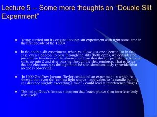
Lecture 5 -- Some more thoughts on “Double Slit Experiment”

1. Lecture 5 -- Some more thoughts on “Double Slit Experiment” • Young carried out his original double-slit experiment with light some time in the first decade of the 1800s. • In the double slit experiment, when we allow just one electron (or in that case, even a photon) to pass through the slits (both open), we consider the probability functions of the electron and say that the this probability function splits up into 2 and after passing through the slits reinforce. That is to say that the electrons pass through both the slits simultaneously (provided that no one is observing). • In 1909 Geoffrey Ingram Taylor conducted an experiment in which he showed that even the feeblest light source - equivalent to "a candle burning at a distance slightly exceeding a mile" - could lead to interference fringes. • This led to Dirac's famous statement that "each photon then interferes only with itself".

2. Further thoughts • Gottfried Möllenstedt and Heinrich Düker -- used an electron biprism - essentially a very thin conducting wire at right angles to the beam - to split an electron beam into two components and observe interference between them. • But in 1961 Claus Jönsson of Tübingen, performed an actual double-slit experiment with electrons for the first time -- demonstrated interference with up to five slits. (Zeitschrift für Physik161 454). • The next milestone - an experiment in which there was just one electron in the apparatus at any one time - was reached by Akira Tonomura at Hitachi in 1989. • They observed the build up of the fringe pattern with a very weak electron source and an electron biprism (American Journal of Physics57 117-120).

3. Double Slit Experiment • The Copenhagen interpretation posits the existence of probability waves which describe the likelihood of finding the particle at a given location. Until the particle is detected at any location along this probability wave, it effectively exists at every point. Thus, when the particle could be passing through either of the two slits, it will actually pass through both, and so an interference pattern results. But if the particle is detected at one of the two slits, then it can no longer be passing through both—its presence must become manifested at one or the other, and so no interference pattern appears. • This is similar to the path integral formulation of quantum mechanics. In the path integral formulation, a particle such as a electron takes every possible path through space-time to get from point A to point B. In the double-slit experiment, point A might be the emitter, and point B the screen upon which the interference pattern appears, and a particle takes every possible path — through both slits at once — to get from A to B. • When a detector is placed at one of the slits, the situation changes, and we now have a different point B. Point B is now at the detector, and a new path proceeds from the detector to the screen. In this eventuality there is only empty space between (B =) A' and the new terminus B', no double slit in the way, and so an interference pattern no longer appears

4. Planck’s Law, PE effect, Thought Experiments • We started with black body radiation – Photoelectric effect—Compton effect --- Net result was that energy is quantised and that light sometimes exhibits wave nature and sometimes exhibits particle nature • Presented the Davison Germer experiment to show that electrons also exhibit wave nature • Presented to you the Stern Gerlach experiment– no classical analogue • Presented to you coupled set of SG experiments and then an analogy with light to give some insight into the mathematics we need to develop • Finally presented to you the heart of quantum mechanics to use the words of a genius

5. Mathematics Now – Linear Vector Space • In our normal Euclidean space we are used to 3 unit vectors • In three dimensions one can express any vector in terms of these vectors • They are said to form a basis • In Stern Gerlach experiment we saw that the spin state of silver atoms could be described in terms of two quantities and we saw we could explain the results using vector algebra, except the two basis vectors had nothing to do with usual vector notion that we have– direction and magnitude • They could be complex also • We must generalise the concept of vectors– throw away some properties adapt some new ones

6. Linear Vector Space • A linear vector space is a collection of objects |1, |2 |3…. |n are called vectors for which the following rules exist • A definite rule for forming the vector sum |v + |w • A definite rule for multiplication by scalars a,b  a|v • Result of either addition or scalar multiplication is another element of space– closure • Scalar multiplication is distributive in the scalars (a+b) |v= a |v + b |v • Multiplicative is distributive in the vector a(|v + |w) = a|v + a |w • Addition is commutative |v + |w = |w + |v • Addition is associative |v + ( |w + |z )= (|v + |w) + |z • There exists a null vector |0 obeying |0 + |v = |v • For every vector |v there exists an inverse under addition |-v such that |v + |-v = |0

7. Linear Vector Space • Conspicuously missing are the requirements that we have grown up with that a vector must have magnitude and direction • The numbers a & b are called field over which the vector space is defined. • If a,b… etc. are all real numbers then it is called a real vector space. If they are complex, they are called complex vector space. • VECTORS themselves ARE NEITHER REAL NOR COMPLEX

8. Linear Vector Space • Having defined what constitutes a vector in our space, briefly examine whether the definition of vectors that we grew up with satisfies this criterion • The rule for addition exists Take the tail of the second arrow and put it on top or head of the first. Connect the tail of the first to the head of the second. • Scalar multiplication  Just stretch the vector • Multiplication by a negative number will change the direction as well as magnitude • Closure property is satisfied. • Addition & scalar multiplication have desired associative & distributive features. • Inverse exists  vector in opposite direction • NULL vector exists  Vector with zero length

9. Linear Vector Space • Now consider a set of 2 X 2 matrices • We know how to add them • Multiplication by scalars is known • Both the above property obey closure. • They are associative as well as distributive • The null matrix has all zeros in it • The inverse of a matrix under addition is matrix with all its elements negated.

10. Linear Independence of a set of vectors • Consider a relation • The set of vectors is said to be linearly independent if such a relation is a trivial one i.e. all ai = 0. • If the set is not linearly independent we say it is linearly dependent. • Not possible to write any member of linearly independent set in terms of others • Two non parallel vectors |u & |u form a linearly independent set. No way we can write one in terms of other. • Equivalently no way to combine them to form a null vector. • A vector space has dimensions n if it can accommodate a maximum of n linearly independent vectors. It will be denoted by If the field is real If the field is complex

11. Definition of a BASIS • Two non parallel vector define a plane. A set of three arrows not in a plane define a 3 dimensional vector space • How about 22 matrix? • Can we accommodate another vector? • Any vector |V in an n-dimensional space can be written as a linear combination of n linearly independent vectors • A set of n linearly independent vectors in n dimensions forms a basis • Any vector can be expanded in terms of these basis vectors • The expansion is unique • To add two vectors one just adds the components • Choosing a basis gives a concrete form to the vectors • While adding two vectors we did not say anything about putting the tail of one vector on the head of other • Multiplication by a scalar multiply its components by the scalar • No explicit rules for actually evaluating the scalar product

12. Inner Product Spaces • Physical properties of vectors aka length and angles in case of arrows • Lets use the dot product • Length of • Cosine of the angle between • How can we use the dot product to define length & angle when the dot product uses length and angle • Main features of the dot product are

13. Pk Pj Linearity Explained Linearity requires that Pj + Pk = Pjk Why do we require Linearity? How does this condition ensure linearity?

14. Inner Product Space for Quantum Mechanics • Inner product in our special space will be denoted by V|W • A vector space with an inner product is called an inner product space • No explicit rule for evaluating the scalar product • The first axiom is sensitive to the order of 2 factors. This is to make V|V real. • Second  Poistive Semidefiniteness- vanishing only if the vector does. It better be because from our generalization we are going to use it to define length • Linearity of inner product when a linear superposition of a|W + b|Z  |aW + bZ appears as a second vector in the scalar product

15. Asymmetry of our space • What if the first factor in the product is a linear superposition • Expresses anti-linearity of the inner product with respect to the first factor in the inner product • The inner product of a linear superposition with another vector is the corresponding superposition of inner product if the superposition occurs in the second factor. • While the superposition with all its coefficients conjugated if the superposition occurs in the first factor. • This assymetry is going to stay with us….

16. Some more properties of Inner Product • Two vectors are orthogonal if the inner product vanishes • The norm of the vector in my vector space is • A set of basis vectors, pairwise orthogonal will be called an orthonormal basis • If we use orthonormal basis only the diagonal terms survive. • We have defined all the properties of inner product but have not specified how to compute it. • We said that the basis is orthonormal if

17. Computing Inner Product • The double sum • Then collapses to • So now you can appreciate why we defined • If it was not defined this way then forget about the norm being positive definite it would not have been real • We have already said that the vector is uniquely defined by its components. Let me denote it by an ordered set of numbers and let me use a column to represent its components i.e. &