Download
1 / 35
350 likes | 521 Views
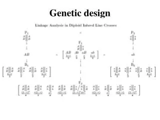
Genetic design. Testing Mendelian segregation. Consider marker A with two alleles A and a Backcross F 2 Aa aa AA Aa aa Observation n 1 n 0 n 2 n 1 n 0 Expected frequency ½ ½ ¼ ½ ¼ Expected number n/2 n/2 n/4 n/2 n/4 The x 2 test statistic is calculated by

E N D
Testing Mendelian segregation Consider marker A with two alleles A and a Backcross F2 Aa aa AA Aa aa Observation n1 n0 n2 n1 n0 Expected frequency ½ ½ ¼ ½ ¼ Expected number n/2 n/2 n/4 n/2 n/4 The x2 test statistic is calculated by x2 = (obs – exp)2 /exp = (n1-n/2)2/(n/2) + (n0-n/2)2/(n/2) =(n1-n0)2/n ~x2df=1, for BC, (n2-n/4)2/(n/4)+(n1-n/2)2/(n/2)+(n0-n/4)2/(n/4)~x2df=2, for F2
Examples Backcross F2 Aa aa AA Aa aa Observation 44 59 43 86 42 Expected frequency ½ ½ ¼ ½ ¼ Expected number 62.5 62.5 42.75 85.5 42.75 The x2 test statistic is calculated by x2 = (obs – exp)2 /exp = (44-59)2/103 = 2.184 < x2df=1 = 3.841, for BC, (43-42.75)2/42.75+(86-85.5)2/85.5+(42-42.75)2/42.75=0.018 < x2df=2 =5.991, for F2 The marker under study does not deviate from Mendelian segregation in both the BC and F2.
Linkage analysis Backcross Parents AABB x aabb ABab F1 AaBb x aabb AB Ab aB abab BC AaBb Aabb aaBb aabb Obs n11 n10 n01 n00 n = nij Freq ½(1-r) ½r ½r ½(1-r) r is the recombination fraction between two markers A and B. The maximum likelihood estimate (MLE) of r is r^ = (n10+n01)/n. r has interval [0,0.5]: r=0 complete linkage, r=0.5, no linkage
Proof of r^ = (n10+n01)/n The likelihood function of r given the observations: L(r|nij) = n!/(n11!n10!n01!n00!) [½(1-r)]n11[½r]n10[½r]n01[½(1-r)]n00 = n!/(n11!n10!n01!n00!) [½(1-r)]n11+n00[½r]n10+n01 log L(r|nij) = C+(n11+n00)log[½(1-r)] +(n10+n01)log[½r] = C + (n11+n00)log(1-r) + (n10+n01)log r + nlog(½) Let the score logL(r|nij)/r = (n11+n00)[-1/(1-r)] +(n10+n01)(1/r) = 0, we have (n11+n00)[1/(1-r)]=(n10+n01)(1/r) r^ = (n10+n01)/n
Testing for linkage BC AaBb aabb Aabb aaBb Obs n11 n00 n10 n01n=nij Freq ½(1-r) ½(1-r) ½r ½r Gamete type nNR= n11+n00 nR= n10+n01 Freq with no linkage ½ ½ Exp ½n ½n x2 = (obs – exp)2/exp = (nNR - nR)2/n ~ x2df=1 Example AaBb aabb Aabb aaBb 49 47 3 4 nNR= 49+47=96 nR= 3 + 4 = 7 n=96+7=103 x2 = (obs – exp)2/exp = (96-7)2/103 = 76.903 > x2df=1 = 3.841 These two markers are statistically linked. r^ = 7/103 = 0.068
Linkage analysis in the F2 BB Bb bb AA Obs n22 n21 n20 Freq ¼(1-r)2½r(1-r)¼r2 Aa Obs n12 n11 n10 Freq ½r(1-r)½(1-r)2+½r2½r(1-r) aa Obs n02 n01 n00 Freq ¼r2½r(1-r)¼(1-r)2 Likelihood function L(r|nij) = n!/(n22!...n00!) [¼(1-r)2]n22+n00[¼r2]n20+n02[½r(1-r)]n21+n12+n10+n01 [½(1-r)2+½r2]n11 Let the score = 0 so as to obtain the MLE of r, but this will be difficult because AaBb contains a mix of two genotype formation types (in the dominator we will have ½(1-r)2+½r2).
I will propose a shortcut EM algorithm for obtain the MLE of r BB Bb bb AA Obs n22 n21 n20 Freq ¼(1-r)2½r(1-r)¼r2 Recombinant 0 1 2 Aa Obs n12 n11 n10 Freq ½r(1-r)½(1-r)2+½r2½r(1-r) Recombinant 1 r2/[(1-r)2+r2] 1 aa Obs n02 n01 n00 Freq ¼r2½r(1-r)¼(1-r)2 Recombinant 2 1 0
Based on the distribution of the recombinants (i.e., r), we have r = 1/(2n)[2(n20+n02)+(n21+n12+n10+n01)+r2/[(1-r)2+r2]n11 (1) = 1/(2n)(2n2R + n1R + n11) where n2R = n20+n02, n1R = n21+n12+n10+n01, n0R = n22+n00. The EM algorithm is formulated as follows E step: Calculate = r2/[(1-r)2+r2] (expected the number of recombination events for the double heterozygote AaBb) M step: Calculate r^ by substituting the calculated from the E step into Equation 1 Repeat the E and M step until the estimate of r is stable
Example BB Bb bb AA n22=20 n21 =17 n20=3 Aa n12 =20n11 =49n10 =19 aa n02=3n01 =21 n00=19 Calculating steps: 1. Give an initiate value for r, r(1) =0.1, 2. Calculate (1)=(r(1))2/[(1- r(1))2+(r(1))2] = 0.12/[(1-0.1)2+0.12] = x; 3. Estimate r using Equation 1, r(2) = y; • Repeat steps 2 and 3 until the estimate of r is stable (converges). The MLE of r = 0.31. How to determine that r has converged? |r(t+1) – r(r)| < a very small number, e.g., e-8
Testing the linkage in the F2 BB Bb bb AA Obs n22=20 n21 =17 n20=3 Exp with no linkage 1/16n 1/8n 1/16n Aa Obs n12 =20n11 =49n10 =19 Exp with no linkage 1/8n ¼n 1/8n aa Obs n02=3n01 =21 n00=19 Exp with no linkage 1/16n 1/8n 1/16n n = nij = 191 x2 = (obs – exp)2/exp ~ x2df=1 = (20-1/16×191)/(1/16×191) + … = a > x2df=1=3.381 Therefore, the two markers are significantly linked.
Log-likelihood ratio test statistic Two alternative hypotheses H0: r = 0 vs. H1: r 0 Likelihood value under H1 L1(r|nij) = n!/(n22!...n00!) [¼(1-r)2]n22+n00[¼r2]n20+n02[½r(1-r)]n21+n12+n10+n01[½(1-r)2+½r2]n11 Likelihood value under H0 L0(r=0.5|nij) = n!/(n22!...n00!) [¼(1-0.5)2]n22+n00[¼0.52]n20+n02[½0.5(1-0.5)]n21+n12+n10+n01[½(1-0.5)2+½0.52]n11 LOD = log10[L1(r|nij)/L0(r=0.5|nij)] = {(n22+n00)2[log10(1-r)-log10(1-0.5)+…} = 6.08 > critical LOD=3
Three-point analysis • Determine a most likely gene order; • Make full use of information about gene segregation and recombination Consider three genes A, B and C. Three possible orders A-B-C, A-C-B, or B-A-C
AaBbCc produces 8 types of gametes (haplotypes) which are classified into four groups Recombinant # between Observation Frequency A and BB and C ABC and abc 0 0 n00=nABC+nabc g00 Abc and abC 0 1 n01=nAbc+nabC g01 aBC and Abc 1 0 n10=naBC+nAbc g10 AbC and aBc 1 1 n11=nAbC+naBc g11 Note that the first subscript of n or g denotes the number of recombinant between A and B, whereas the second subscript of n or g denotes the number of recombinant between B and C (assuming order A-B-C)
Matrix notations Markers B and C Markers A and B Recombinant Non-recombinant Total Recombinant n11 n10 Non-recombinant n01 n00 Total n Recombinant g11 g10 rAB Non-recombinant g01 g00 1-rAB Total rBC 1-rBC 1 What is the recombination fraction between A and C? rAC = g01 + g10 Thus, we have rAB = g11 + g10 rBC = g11 + g01 rAC = g01 + g10
The data log-likelihood (complete data, it is easy to derive the MLEs of gij’s) log L(g00, g01, g10, g11| n00, n01, n10, n11, n) = log n! – (log n00! + log n01! + log n10! + log n11!) + n00 log g00 + n01 log g01 + n10 log g10+ n11 log g11 The MLE of gij is: gij^ = nij/n Based on the invariance property of the MLE, we obtain the MLE of rAB, rAC and rBC. A relation: 0 g11 = ½(rAB + rBC - rAC) rAC rAB + rBC 0 g10 = ½(rAB - rBC + rAC) rBC rAB + rAC 0 g01 = ½(-rAB + rBC + rAC) rAB rAC + rBC
Advantages of three-point (and generally multi-point) analysis • Determine the gene order, • Increase the estimation precision of the recombination fractions (for partially informative markers).
Real-life example – AoC/oBo ABC/ooo Eight groups of offspring genotypes A_B_C_ A_B_cc A_bbC_ A_bbcc aaB_C_ aaV_cc aabbC_ aabbcc Obs. 28 4 12 3 1 8 2 2 Order A - B - C Two-point analysis 0.380.386 0.390.418 0.180.056 Three-point analysis 0.200.130 0.200.130 0.200.059
Multilocus likelihood – determination of a most likely gene order • Consider three markers A, B, C, with no particular order assumed. • A triply heterozygous F1 ABC/abc backcrossed to a pure parent abc/abc Genotype ABC or abc ABc or abC Abc or aBC AbC or aBc Obs. n00 n01 n10 n11 Frequency under Order A-B-C (1-rAB)(1- rBC) (1-rAB) rBC rAB(1- rBC) rAB rBC Order A-C-B (1-rAC)(1- rBC) rAC rBC rAC(1-rBC)(1-rAC)rBC Order B-A-C (1-rAB)(1- rAC) (1-rAB) rAC rABrAC rAB(1-rAC) rAB = the recombination fraction between A and B rBC = the recombination fraction between B and C rAC = the recombination fraction between A and C
It is obvious that rAB = (n10 + n11)/n rBC = (n01 + n11)/n rAC = (n01 + n10)/n What order is the mostly likely? LABC (1-rAB)n00+n01 (1-rBC)n00+n10 (rAB)n10+n11 (rBC)n01+n11 LACB (1-rAC)n00+n11 (1-rBC)n00+n10 (rAC)n01+n10 (rBC)n01+n11 LBAC (1-rAB)n00+n01 (1-rAC)n00+n11 (rAB)n10+n11 (rAC)n01+n10 According to the maximum likelihood principle, the linkage order that gives the maximum likelihood for a data set is the best linkage order supported by the data. This can be extended to include many markers for searching for the best linkage order.
Map function • Transfer the recombination fraction (non-additivity) between two genes into their corresponding genetic map distance (additivity) • Map distance is defined as the mean number of crossovers • The unit of map distance is Morgan (in honor of T. H. Morgan who obtained the Novel prize in 1930s) • 1 Morgan or M = 100 centiMorgan or cM
The Haldane map function (Haldane 1919) Assumptions: • No interference (the occurrence of one crossover is independent of that of next) • Crossover events follow the Poisson distribution. Consider three markers with an order A-B-C A triply heterozygous F1 ABC/abc backcrossed to a pure parent abc/abc Event Gamete Frequency No crossover ABC or abc (1-rAB)(1-rBC) Crossover between B&C ABc or abC (1-rAB)rBC Crossover between A&B Abc or aBC rAB(1-rBC) Crossovers between A&B and B&C AbC or aBc rABrBC The recombination fraction between A and C is expected to be rAC = (1-rAB)rBC + rAB(1-rBC) = rAB+rBC-2rABrBC (1-2rAC)=(1-2rAB)(1-2rBC)
Map distance: A genetic length (map distance) x of a chromosome is defined as the mean number of crossovers. Poisson distribution (x = genetic length): Crossover event 0 1 2 3 … t … Probability e-x xe-x x2e-x x3e-x … xte-x … 2! 3! t!
The value of r (recombination fraction) for a genetic length of x is the sum of the probabilities of all odd numbers of crossovers: r = e-x(x1/1! + x3/3! + x5/5! + x7/7! + …) = ½(1- e-2x) x = -ln(1-2r) We have xAC = xAB + xBC for a given order A-B-C, but generally, rAC rAB + rBC
Proof of xAC = xAB + xBC For order A-B-C, we have rAB = ½(1- e-2xAB), rBC = ½(1- e-2xBC), rAC = ½(1- e-2xAC) rAC = rAB + rBC – 2rABrBC = ½(1- e-2xAB) + ½(1- e-2xBC) - 2 ½(1- e-2xAB) ½(1- e-2xBC) = ½[1- e-2xAB +1- e-2xBC-1+ e-2xAB + e-2xBC - e-2xAB e-2xBC = ½(1- e-2(xAB+xBC)) = ½(1- e-2xAC), which means xAC = xAB + xBC
The Kosambi map function (Kosambi 1943) The Kosambi map function is an extension of the Haldane map function For gene order A-B-C [1] rAC = rAB + rBC – 2rABrBC [2] rAC rAB + rBC, for small r’s [3] rAC rAB + rBC – rABrBC, for intermediate r’s The Kosambi map function attempts to find a general expression that covers all the above relationships
Map Function Haldane Kosambi x = -½ln(1-2r) ¼ln(1+2r)/(1-2r) r = ½(1-e-2x) ½(e2x-e-2x)/(e2x+e-2x) rAB = rA+rB-2rArB (rA+rB)/(1+4rArB) Reference Ott, J, 1991 Analysis of Human Genetic Linkage. The Johns Hopkins University Press, Baltimore and London
Construction of genetic maps • The Lander-Green algorithm -- a hidden Markov chain • Genetic algorithm
Linkage analysis between two dominant markers Dominant marker - AA and AO cannot be separated from each other in phenotype. But both of them are different from third genotype OO. Two codominant markers A and B 1/4AA + 1/2Aa + 1/4aa = 1AA: 2Aa: 1aa 1/4BB + 1/2Bb + 1/4bb = 1BB: 2Bb: 1bb Two dominant markers A and B Mix(1/4AA + 1/2AO): 1/4OO = 3A_ : 1OO Mix(1/4BB + 1/2BO): 1/4OO = 3B_ : 1OO
Let r be the recombination fraction between the two markers For two codominant markers, we have 9 (=3x3) groups of genotypes in the F2, whose genotype frequencies are expressed, in matrix notation, as AA Aa aa total BB ¼(1-r)2 ½r(1-r) ¼r2 1/4 Bb ½r(1-r) ½[(1-r)2+r2] ¼r(1-r) 1/2 bb ¼r2 ½r(1-r) ¼(1-r)2 1/4 Total 1/4 1/2 1/4 1
For one codominant (B) and one dominant marker (A), 9 groups of genotypes will be collapsed into 6 (=32) distinguishable groups: A_ aa total BB ¼(1-r)2 + ½r(1-r) ¼r2 1/4 Bb ½r(1-r) + ½[(1-r)2+r2] ¼r(1-r) 1/2 bb ¼r2 + ½r(1-r) ¼(1-r)2 ¼ Total 3/4 1/4 1
For two dominant markers, 9 groups of genotypes will be collapsed into 4 (=22) distinguishable groups. The 2x2 probability matrix is A_ aa total B_ ¼(1-r)2 + ½r(1-r) ¼r2 + ½r(1-r) + ½[(1-r)2+r2] + ¼r(1-r) 3/4 bb ¼r2 + ½r(1-r) ¼(1-r)2 1/4 Total 3/4 1/4 1
Observations counted from the poplar data set provided: A_ aa Total B_ n1 n2 bb n3 n4 Total n
Expected numbers of recombinant gametes (the number of r) A_ aa B_ c1 c2 bb c2 0 where c1 = [2½r2+1r(1-r)]/[½r2+r(1-r)+¾(1-r)2] (1) c2 = [2¼r2+1½r(1-r)]/[¼r2+½r(1-r)] (2) Based on the definition of r (the proportion of recombinant gametes over all gametes), we have r^ = (c1n1 + c2n2 + c3n3) /2n (3) Equations (1) and (2) are for the E step, whereas Equation (3) is for the M step.