Download
1 / 62
620 likes | 773 Views
CMS ECAL calibration and Search for the Standard Model H gg Yong Yang, Caltech Fermilab RA candidate talk, Nov 27 2012. Introduction. A great success of the Standard Model so far. Higgs mechanism, giving mass to W, Z boson and fermions. Predicted a Higgs boson, the last particle

E N D
CMS ECAL calibration and Search for the Standard Model Hgg Yong Yang, Caltech Fermilab RA candidate talk, Nov 27 2012
Introduction • A great success of the Standard Model so far. • Higgs mechanism, giving mass to W, Z boson and fermions. • Predicted a Higgs boson, the last particle to be firmly confirmed. • Both CMS and ATLAS experiments observed a new particle around 125 GeV, statistically consistent with SM Higgs boson.
Large Hadron Collider • Proton-proton collider at √s = 7, 8 TeV (design 14 TeV) • Built to answer most fundamental open questions in physics: • Interactions and forces, deep structure of space and time • Higgs mechanism in Standard model, new physics. • Excellent performance in first 2 years of running, peak instantaneous luminosity: • 2011, 4 x 1033 cm-2s-1 • 2012, 7.6 x 1033 cm-2s-1 • Design, 1034 cm-2s-1 27 km circumference 50-175 m underground
Analyzed data Expected 25 fb-1 by end of pp running this year 2011’s data used in majority of this talk. Latest Hggresults upto July 2012
Pileups • pileups: simultaneous inelastic interactions • multiple vertices: challenge for Hgg • pileup energies added into a cone around the object: less “isolated”. g Vertex Isolation energy energy from pileup g
Compact Muon Solenoid • Modular design Pre-assembled • Powerful 3.8 Tesla magnets Tracking • Crystal ECAL high resolution • Hermetic calorimeter Jet and missing ET • Muon system (tracker + muon detectors) resolution <10% at TeV P PT q z axis (beam line) x-y plane ,f in x-y plane
Higgs boson production at LHC • Higgs boson production modes at the LHC: Cross section [pb] @ 7TeV Gluon-gluon fusion Vector Boson fusion Uncertainty ~15% top-top fusion Higgs bremsstrahlung • Cross Section @ 7 / 8 / 14 TeV @ 125 GeV: 17.5 / 22.3 / 57.0 pb
Hgg decay Uncertainty: input parameters + missing high orders • In the mass rang of interest, from 110 to 150 GeV, small branching ratio ~ 0.2%. • However, competitive sensitivity due to the narrow resonance.
Challenge of Hgg searches • Simple final states: two high pT photons. • Simple discriminating variable: invariant mass of two photons. • Resonance on top of large background. • S/B at 125GeV ~ 1/20. • Analysis is all about the mass resolution: The main challenge: photon energy resolution (measured in ECAL) Signal x 10.
CMS ECAL: 76K Crystals EndCap Barrel Crystals Test beam SuperModule • Homogeneous, compact, and fine grain PWO4 crystal calorimeter • Barrel (|h|<1.5): 61,200 PWO4 crystals + two endcaps ( 1.5<|h|<3, 2x7324 crystals). • Advantage: Intrinsic energy resolution (0.5% for E>100 GeV) • Challenges: achieving this goal in-situ.
ECAL energy measurement CMS measures electron/photon energy as One crystal (channel) • ADCi : single channel amplitude • G: global ECAL energy scale from amplitude to energy. • ci: intercalibration constant for each channel. • LCi: time-dependent correction from laser monitoring system. • f(e/g): particle (object level) energy correction.
Why challenging? • In real CMS detector of ECAL • Response non-uniformity, 15%-25% channel-to-channel variation. • Channel-to-channel Intercalibration • Crystals suffers from dose rate dependent radiation damages, resulting in transparency loss (beam on) and recovery (beam off) • Laser monitoring and correction • Material in front of ECAL, gaps between crystals, shower containment, pileup. • Object level (cluster) energy correction
ECAL energy inter-calibration • Precalibration using test beam, cosmic rays, radiation source prior to installation to precision 0.5% for 20% barrel crystals, and to 1- few % for the rest. • CMS in-situ strategies to equalize the channel-to-channel response variations. e: E/p π0,gg f-symmetry
π0,gg calibration • Principle: use invariant mass of two photons to equalize the energy responses of each crystal. • Main challenges: • To collect enough π0 decays (barrel: 3000 π0 / crystal) to repeat intercalibration every few weeks. Need a dedicated calibration trigger. • Significant extrapolation in energy from calibration sample to Higgs sample. Need explicit validation of calibration performance at high energy. Intercalibration different channels E π0,gg (2-10 GeV) Hgg (50-300 GeV)
π0,gg calibration trigger Data after L1 Triggers Calibration Dedicated online farm ~7 kHz ~50 kHz ~2 ms / event 4-6 MB /s • Main Problem: high output rate required • Saturates HLT processing and output bandwidth (total standard HLT output rate ~300Hz) • Solution: • Restrict to localized ECAL crystal-level information near L1 EG seeds . • Simple selections: pT(g)>1.0 GeV, E4/E9>0.83. • Final selected π0 candidate reduces output to only 20-30 crystals per event
Online selections • Simple selections on pT(g) and pT(gg) , shower shape and isolation (optimized to reject conversion) • only ECAL local-variables used.
Intercalibration method • Iterative method is used to derive the intercalibration constant. (L3 method, see backup) • Adjust the constant step-by-step till it converges channel 1 channel 1 channel 1 channel 2 channel 2 channel 2 channel N channel N channel N Step0 (precalibration) Step1 … Step final Note that N is large (61k for barrel, 15k for endcaps) • CPU consumption is significant.
Improve calibration procedure Module gaps • Cluster containment has dependence on h and j • This dependence introduces energy measurement bias • Correcting for these biases improves the calibration precision by a factor of two.
Intercalibration result (example) cπ0 for each channel • i crystal index, π0 calibration constant is a correction for precalibration (or the current calibration) • In some supermodules, less corrections better precalibrated • white areas dead channels • 3 best precalibrated supemodules used as the reference to study the π0 calibration precision. One supermodule ( 85 x 20 crystals)
Calibration precision (2011) • The single-crystal calibration precision is dominated by π0() method for |h|<2.0 • The region of |h|<1.0 calibrated to 0.5% and is the most important region for Hggsearch
Laser monitoring • Response drops due to transmission loss caused by radiation damage. • Continuous laser monitoring and correction: one measurement of all crystals per 20 minutes.
Laser-monitoring correction • Average signal loss of 2.5% in the barrel, and 10% in the endcaps • After correction, the energy scale (E/p) is stable with 0.1% and 0.5% for barrel and endcaps.
Validation of in-situ calibration Ze+e- • In-situ intercalibration and laser corrections are validated at high energy using Ze+e- data. • Significant improvement on the ECAL energy resolution over precalibrations.
Impact on Hgg search 95% CL limits on s/sSM Precalibration Precalibration + Laser correction In-situ calibration + Laser correction • 38% improvement on the search sensitivity in terms of the exclusion limit due to in-situ intercalibration and laser monitoring correction.
Photon energy correction Ze+e- • The raw clustered energy has dependencies on many factors, for example: crystal gaps, tracker material, pileup • These non-uniformities degrades resolution • CMS standard correction, correcting dependence on a few variables one after another, improves the performance but is sub-optimal.
Multivariate-based correction • The non-uniformities in response, and correlations among dependent variables can be very complicated. • Therefore a multivariate regression technique significantly improves the energy correction.
Regression analysis • A general machine learning technique: • generates a map from a list of input variables to some output • Map is optimized for some particular goal • In our case we optimize for the target Etrue/Ereco • Important to choose well simulated input variables • Otherwise performance in data may degrade Multidimensional minimization problem
Improve Hggsearch sensitivity • Resolution improvement of the MVA-based correction is validated with Ze+e- data. • Absolute scale is also more correct. • 14% improvement on the Hggsearch sensitivity.
Validation of energy resolution • The Hgg photon energy resolution are modeled from MC simulation, and thus needs to be validated with data. • Comparison of the Ze+e- mass resolution between data and MC leads to correction (smearing) of the energy in simulation. • Maximum likelihood fit r9 = E3x3/Ecluster
Photon identification • Large reducible g+jet, jet+jet backgrounds are reduced by cutting on a few variables: • Isolation rAeff is for “pileup” subtraction. • H/E: Hadronic energy (HCAL) / photon energy (ECAL). almost all photon energies are deposited in ECAL only ( 25 radiation length). • Transverse shape of electromagnetic shower. (narrow for real g, wider for fake g) π0 (misidentified asg) π,k.. g
Example N-1 distributions • Selection cuts are separately tuned for photons in 4 “categories”: Barrel or endcaps + r9>0.94 or r9<0.94. • Difference in selection efficiency due to disagreement between data and MC is corrected using Z e+e-.
Event classification • Search sensitivity is improved by splitting all events into different classes according to mass resolution and signal-over-background. Best Resolution Best S/B
Hgg parameterized model • Signal models: 1-3 Gaussians, depending on the category, to well describe both the core and tail of the distributions. • Models separately built for events with or without a correct vertex, in each event category. • Limited mass points simulated. Interpolation for other mass points (right plot).
Background fit on data • Background fit for first two event categories and the expected signal Hgg distribution at 120 GeV. • Use the functional form (5th order bernstein polynomial) that minimizes the bias with respect to a set of possible functional forms (backup). • conservative estimate of the sensitivity
Background fit on data (II) • Background fit for 3rd and 4th event categories.
Background fit on data (III) The excess • Background fit for di-jet (left, 2nd order Bernstein polynomial) and combined categories.
Systematic uncertainties Varying resolution Varying scale • H gg signal shape (sum of Gaussians) is affected by the imprecisely known energy resolution and scale, measured with Ze+e- . • Signal yield is affected by cross section and efficiency uncertainties.
Statistical Interpretation • Statistical analysis gives the quantitative statement of the search results. Two approaches in high energy experiments, differ in the way to interpret “Probability”: • Bayesian: a measure of degree of belief • Frequentist. the frequency of occurrence • CMS and ATLAS have adopted a fully frequentist based method called “CLs-LHC”. • Based on likelihood ratio. • Systematic uncertainties profiling the nuisance parameters. ( add penalty terms in likelihoods) • Allows for comparison and combination • Exist asymptotic approximation, fast computation.
Exclusion limits • 95% CL upper cross section limit (unit of Standard Model H gg cross section) • SM Higgs boson at given mass is excluded if the observed value is < 1. • Peak indicates event excess over background prediction.
Quantifying the significance • The probability of excess due to background statistical fluctuation. • Local significance: 3.3 standard deviation at 123 GeV • Global significance is 2.0 s, taking into account the unknown mass from 110 to 150 GeV.
Lates results from CMS • Categories combined using S/(S+B). • > 5s significance at 125 GeV. 127-600 GeV is all excluded at high significanceunder Standard Model hypothesis.
Signal strength (s/sSM) 2012 HCP • H gg: 1.6 +/- 0.4 [July 2012] • Production is statistically consistent with a Standard Model Higgs boson 0.88 ± 0.21
Summary • CMS ECAL calibration and correction are crucial to reach the optimal performance, played an important role for the discovery in 2012, in particularly important for Hgg. • π0,gg + f-symmetry + electron in-situ channle-by-channel energy intercalibration. • Laser monitoring and correction for crystal transparency variations. • Object-level multivariate energy correction. • Continued to be very important for ECAL performance and physics at CMS. • Also more challenging at higher luminosities.
ECAL energy clustering • Measured photon energy has dependence on shape of shower • Particularly for converted photons • CMS uses a supercluster algorithm to collect energy from conversion pairs • Converted photons may be identified using the variable r9 = E3x3/Esc
The resolution performance • Central barrel (less material), high r9 (less conversions) • the resolution approaches to 1% at high energies (recall that 0.55% of design) • Main reasons: • imperfect energy correction for conversion, crystal gaps, etc. • imperfect in-situ laser correction • In other categories, worse results due to larger material. Material budget tracker pixel
Hgg vertex identification 1.72 3.10 • The track activities in the best category of Hgg events with two un-converted photons are similar as these pileup events. • A multivariate vertex ID is developed to improve the ID efficiency for low pT Higgs events and larger pileups. • Using , balance and asymmetry of di-photon pT and other tracks, photon conversion significance.
Vertex ID improvement • 10% improvement for events with low pT or larger number of vertices.
Improve Hggsearch sensitivity • 4% improvement on the Hggsearch sensitivity from the improvement on the vertex ID efficiency.