Exploring Computational Social Choice: Voting Rules and Aggregation Mechanisms
This document provides an overview of computational social choice, focusing on various voting rules and their applications in decision-making processes. It discusses the fundamental frameworks for ranking alternatives, the role of voting mechanisms in determining winners, and the complexity of strategic voting. Key examples of voting rules, such as Borda count and Single Transferable Vote, are explained, along with their implications for collective decision-making. Additional insights into axiomatic approaches and combinatorial voting scenarios are presented, emphasizing the richness of this interdisciplinary field.


Exploring Computational Social Choice: Voting Rules and Aggregation Mechanisms
E N D
Presentation Transcript
thanks to: Computational Social Choice Lirong Xia Ph.D. Duke CS 2011, now CIFellow @ Harvard Vincent Conitzer Duke University 2012 Summer School on Algorithmic Economics, CMU
A few shameless plugs • General: • New journal: ACM Transactions on Economics and Computation (ACM TEAC) • Computational Social Choice: • intro chapter: F. Brandt, V. Conitzer and U. Endriss, Computational Social Choice. • community mailing list: • https://lists.duke.edu/sympa/subscribe/comsoc
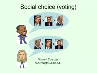
Voting over alternatives voting rule (mechanism) determines winner based on votes > > • Can vote over other things too • Where to go for dinner tonight, other joint plans, … > >
Voting (rank aggregation) • Set of m candidates (aka. alternatives, outcomes) • n voters; each voter ranks all the candidates • E.g., for set of candidates {a, b, c, d}, one possible vote is b > a > d > c • Submitted ranking is called a vote • A voting rule takes as input a vector of votes (submitted by the voters), and as output produces either: • the winning candidate, or • an aggregate ranking of all candidates • Can vote over just about anything • political representatives, award nominees, where to go for dinner tonight, joint plans, allocations of tasks/resources, … • Also can consider other applications: e.g., aggregating search engines’ rankings into a single ranking
Outline • Example voting rules • How might one choose a rule? • Axiomatic approach • MLE approach • Hard-to-compute rules • Strategic voting • Using computational hardness to prevent manipulation and other undesirable behavior • Elicitation and communication complexity • Combinatorial alternative spaces
Example voting rules • Scoring rules are defined by a vector (a1, a2, …, am); being ranked ith in a vote gives the candidate ai points • Plurality is defined by (1, 0, 0, …, 0) (winner is candidate that is ranked first most often) • Veto (or anti-plurality) is defined by (1, 1, …, 1, 0) (winner is candidate that is ranked last the least often) • Borda is defined by (m-1, m-2, …, 0) • Plurality with (2-candidate) runoff: top two candidates in terms of plurality score proceed to runoff; whichever is ranked higher than the other by more voters, wins • Single Transferable Vote (STV, aka. Instant Runoff): candidate with lowest plurality score drops out; if you voted for that candidate, your vote transfers to the next (live) candidate on your list; repeat until one candidate remains • Similar runoffs can be defined for rules other than plurality
Pairwise elections two votes prefer Obama to McCain > > > two votes prefer Obama to Nader > > > two votes prefer Nader to McCain > > > > >
Condorcet cycles two votes prefer McCain to Obama > > > two votes prefer Obama to Nader > > > two votes prefer Nader to McCain > ? > > “weird” preferences
Pairwise election graphs • Pairwise election between a and b: compare how often a is ranked above b vs. how often b is ranked above a • Graph representation: edge from winner to loser (no edge if tie), weight = margin of victory • E.g., for votes a > b > c > d, c > a > d > b this gives b a 2 2 2 c d
Voting rules based on pairwise elections • Copeland: candidate gets two points for each pairwise election it wins, one point for each pairwise election it ties • Maximin (aka. Simpson): candidate whose worst pairwise result is the best wins • Slater: create an overall ranking of the candidates that is inconsistent with as few pairwise elections as possible • NP-hard! • Cup/pairwise elimination: pair candidates, losers of pairwise elections drop out, repeat • Ranked pairs (Tideman): look for largest pairwise defeat, lock in that pairwise comparison, then the next-largest one, etc., unless it creates a cycle
Even more voting rules… • Kemeny: create an overall ranking of the candidates that has as few disagreements as possible (where a disagreement is with a vote on a pair of candidates) • NP-hard! • Bucklin: start with k=1 and increase k gradually until some candidate is among the top k candidates in more than half the votes; that candidate wins • Approval (not a ranking-based rule): every voter labels each candidate as approved or disapproved, candidate with the most approvals wins
Choosing a rule • How do we choose a rule from all of these rules? • How do we know that there does not exist another, “perfect” rule?
Condorcet criterion • A candidate is the Condorcet winner if it wins all of its pairwise elections • Does not always exist… • … but the Condorcet criterion says that if it does exist, it should win • Many rules do not satisfy this • E.g. for plurality: • b > a > c > d • c > a > b > d • d > a > b > c • a is the Condorcet winner, but it does not win under plurality
Distance rationalizability • Dodgson: candidate wins that can be made Condorcet winner with fewest swaps of adjacent alternatives in votes • NP-hard! • Generalization of this idea: • Define consensus profiles with a clear winner • Define distance function between profiles • Rule: find the closest consensus profile, choose its winner • Another example: consensus = unanimity on first-ranked alternative; distance = how many votes are different. This gives…? • More on distance rationalizability: see Elkind, Faliszewski, Slinko COMSOC 2010 , also Baigent 1987, Meskanen and Nurmi 2008, …
Majority criterion • If a candidate is ranked first by a majority (> ½) of the votes, that candidate should win • Relationship to Condorcet criterion? • Some rules do not even satisfy this • E.g., Borda: • a > b > c > d > e • a > b > c > d > e • c > b > d > e > a • a is the majority winner, but it does not win under Borda
Monotonicity criteria • Informally, monotonicity means that “ranking a candidate higher should help that candidate,” but there are multiple nonequivalent definitions • A weak monotonicity requirement: if • candidate w wins for the current votes, • we then improve the position of w in some of the votes and leave everything else the same, • then w should still win. • E.g., STV does not satisfy this: • 7 votes b > c > a • 7 votes a > b > c • 6 votes c > a > b • c drops out first, its votes transfer to a, a wins • But if 2 votes b > c > a change to a > b > c, b drops out first, its 5 votes transfer to c, and c wins
Monotonicity criteria… • A strong monotonicity requirement: if • candidate w wins for the current votes, • we then change the votes in such a way that for each vote, if a candidate c was ranked below w originally, c is still ranked below w in the new vote • then w should still win. • Note the other candidates can jump around in the vote, as long as they don’t jump ahead of w • None of our rules satisfy this
Independence of irrelevant alternatives • Independence of irrelevant alternatives criterion: if • the rule ranks a above b for the current votes, • we then change the votes but do not change which is ahead between a and b in each vote • then a should still be ranked ahead of b. • None of our rules satisfy this
Arrow’s impossibility theorem [1951] • Suppose there are at least 3 candidates • Then there exists no rule that is simultaneously: • Pareto efficient (if all votes rank a above b, then the rule ranks a above b), • nondictatorial (there does not exist a voter such that the rule simply always copies that voter’s ranking), and • independent of irrelevant alternatives
Muller-Satterthwaite impossibility theorem [1977] • Suppose there are at least 3 candidates • Then there exists no rule that simultaneously: • satisfies unanimity (if all votes rank a first, then a should win), • is nondictatorial (there does not exist a voter such that the rule simply always selects that voter’s first candidate as the winner), and • is monotone (in the strong sense).
Manipulability • Sometimes, a voter is better off revealing her preferences insincerely, aka. manipulating • E.g., plurality • Suppose a voter prefers a > b > c • Also suppose she knows that the other votes are • 2 times b > c > a • 2 times c > a > b • Voting truthfully will lead to a tie between b and c • She would be better off voting, e.g., b > a > c, guaranteeing b wins • All our rules are (sometimes) manipulable
Gibbard-Satterthwaite impossibility theorem • Suppose there are at least 3 candidates • There exists no rule that is simultaneously: • onto (for every candidate, there are some votes that would make that candidate win), • nondictatorial (there does not exist a voter such that the rule simply always selects that voter’s first candidate as the winner), and • nonmanipulable (strategy-proof)
Objectives of social choice • OBJ1: Compromise among subjective preferences • OBJ2: Reveal the “truth”
The MLE approach to voting [dating back to Condorcet 1785] • Given the “correct outcome” o • each vote is drawn conditionally independently given o, according to Pr(V|o) • o can be a winning ranking or a winning alternative • The MLE rule: For any profile P, • The likelihood of P given o: L(P|o)=Pr(P|o)=∏V∈P Pr(V|o) • The MLE as rule is defined as MLEPr(P)=argmaxo∏V∈PPr(V|o) “Correct” outcome …… Vote 1 Vote 2 Vote n
Two alternatives • One of the two alternatives {A,B} is the “correct” winner; this is not directly observed • Each voter votes for the correct winner with probability p > ½, for the other with 1-p (i.i.d.) • The probability of a particular profile in which a is the number of votes for A and b that for B (a+b=n)... • ... given that A is the correct winner is pa(1-p)b • ... given that B is the correct winner is pb(1-p)a • Maximum likelihood estimate: whichever has more votes (majority rule)
Independence assumption ignores social network structure Voters are likely to vote similarly to their neighbors!
What should we do if we know the social network? • Argument 1: “Well-connected voters benefit from the insight of others so they are more likely to get the answer right. They should be weighed more heavily.” • Argument 2: “Well-connected voters do not give the issue much independent thought; the reasons for their votes are already reflected in their neighbors’ votes. They should be weighed less heavily.” • Argument 3: “We need to do something a little more sophisticated than merely weigh the votes (maybe some loose variant of districting, electoral college, or something else...).”
Factored distribution • Let Vv be v’s vote, N(v) the neighbors of v • Associate a function fv(Vv,VN(v) | c) with node v (for c as the correct winner) • Given correct winner c, the probability of the profile is Πv fv(Vv,VN(v) | c) • Assume: fv(Vv,VN(v) | c) = gv(Vv | c) hv(Vv,VN(v)) • Interaction effect is independent of correct winner
Example (2 alternatives, 2 connected voters) • gv(Vv=c| c) = .7, gv(Vv= -c| c) = .3 • hvv’(Vv=c, Vv’=c) = 1.142, hvv’(Vv=c, Vv’=-c) = .762 • P(Vv=c| c) = P(Vv=c, Vv’=c| c) + P(Vv=c, Vv’=-c| c) = (.7*1.142*.7*1.142 + .7*.762*.3*.762) = .761 • (No interaction: h=1, so that P(Vv=c| c) = .7)
Social network structure does not matter! [C., Math. Soc. Sci. 2012] • Theorem. The maximum likelihood winner does not depend on the social network structure. (So for two alternatives, majority remains optimal.) • Proof. arg maxcΠv fv(Vv,VN(v) | c) = arg maxcΠv gv(Vv | c) hv(Vv,VN(v)) = arg maxcΠv gv(Vv | c).
An MLE model for >2 alternatives [dating back to Condorcet 1785] • Correct outcome is a ranking W , p>1/2 • MLE = Kemeny rule [Young ‘88, ‘95] • Pr(P|W) = pnm(m-1)/2-K(P,W) (1-p) K(P,W)= • The winning rankings are insensitive to the choice of p (>1/2) p c≻d in V c≻d in W d≻c in V 1-p Pr( b≻c≻a|a≻b≻c ) = p (1-p) p (1-p)2 (1-p)
A variant for partial orders[Xia & C. IJCAI-11] • Parameterized by p+ > p- ≥0 (p+ +p- ≤1) • Given the “correct” ranking W, generate pairwise comparisons in a vote VPO independently c≻d in VPO p+ p- d≻c in VPO c≻d in W 1-p+-p- not comparable
MLE for partial orders… [Xia & C. IJCAI-11] • In the variant to Condorcet’s model • Let T denote the number of pairwise comparisons in PPO • Pr(PPO|W) = (p+)T-K(PPO,W) (p-)K(PPO,W)(1-p+-p-)nm(m-1)/2-T • The winner is argminWK(PPO,W) =
Which other common rules are MLEs for some noise model?[C. & Sandholm UAI’05; C., Rognlie, Xia IJCAI’09] • Positional scoring rules • STV - kind of… • Other common rules are provably not • Consistency: if f(V1)∩ f(V2) ≠ Ø then f(V1+V2) = f(V1)∩ f(V2) (f returns rankings) • Every MLE rule must satisfy consistency! • Incidentally: Kemeny uniquely satisfies neutrality, consistency, and Condorcet property [Young & Levenglick 78]
Correct alternative • Suppose the ground truth outcome is a correct alternative (instead of a ranking) • Positional scoring rules are still MLEs • Consistency: if f(V1)∩ f(V2) ≠ Ø then f(V1+V2) = f(V1)∩ f(V2) (but now f produces a winner) • Positional scoring rules* are the only voting rules that satisfy anonymity, neutrality, and consistency![Smith ‘73, Young ‘75] • * Can also break ties with another scoring rule, etc. • Similar characterization using consistency for ranking?
Kemeny & Slater • Closely related • Kemeny: • NP-hard [Bartholdi, Tovey, Trick 1989] • Even with only 4 voters [Dwork et al. 2001] • Exact complexity of Kemeny winner determination: complete for Θ_2^p [Hemaspaandra, Spakowski, Vogel 2005] • Slater: • NP-hard, even if there are no pairwise ties [Ailon et al. 2005, Alon 2006, C. 2006, Charbit et al. 2007]
Kemeny on pairwise election graphs • Final ranking = acyclic tournament graph • Edge (a, b) means a ranked above b • Acyclic = no cycles, tournament = edge between every pair • Kemeny ranking seeks to minimize the total weight of the inverted edges Kemeny ranking pairwise election graph 2 2 b a b a 2 4 2 2 10 c d c d 4 (b > d > c > a)
Slater on pairwise election graphs • Final ranking = acyclic tournament graph • Slater ranking seeks to minimize the number of inverted edges Slater ranking pairwise election graph b a b a c d c d (a > b > d > c) Minimum Feedback Arc Set problem (on tournament graphs, unless there are ties)
An integer program for computing Kemeny/Slater rankings • y(a, b) is 1 if a is ranked below b, 0 otherwise • w(a, b) is the weight on edge (a, b) (if it exists) • in the case of Slater, weights are always 1 • minimize: ΣeE we ye • subject to: • for all a, b V, y(a, b) + y(b, a) = 1 • for all a, b, c V, y(a, b) +y(b, c) + y(c, a) ≥ 1
A few references for computing Kemeny / Slater rankings • Ailon et al. Aggregating Inconsistent Information: Ranking and Clustering. STOC-05 • Ailon. Aggregation of partial rankings, p-ratings and top-m lists. SODA-07 • Betzler et al. Partial Kernelization for Rank Aggregation: Theory and Experiments. COMSOC 2010 • Betzler et al. How similarity helps to efficiently compute Kemeny rankings. AAMAS’09 • Brandt et al. On the fixed-parameter tractability of composition-consistent tournament solutions. IJCAI’11 • C. Computing Slater rankings using similarities among candidates. AAAI’06 • C. et al. Improved bounds for computing Kemeny rankings. AAAI’06 • Davenport and Kalagnanam. A computational study of the Kemeny rule for preference aggregation. AAAI’04 • Meila et al. Consensus ranking under the exponential model. UAI’07
Dodgson • Recall Dodgson’s rule: candidate wins that requires fewest swaps of adjacent candidates in votes to become Condorcet winner • NP-hard to compute an alternative’s Dodgson score [Bartholdi, Tovey, Trick 1989] • Exact complexity of winner determination: complete for Θ_2^p [Hemaspaandra, Hemaspaandra, Rothe 1997] • Several papers on approximating Dodgson scores[Caragiannis et al. 2009, Caragiannis et al. 2010] • Interesting point: if we use an approximation, it’s a different rule! What are its properties? Maybe we can even get better properties?
Inevitability of manipulability • Ideally, our mechanisms are strategy-proof, but may be too much to ask for • Gibbard-Satterthwaite theorem: Suppose there are at least 3 alternatives There exists no rule that is simultaneously: • onto (for every alternative, there are some votes that would make that alternative win), • nondictatorial, and • strategy-proof • Typically don’t want a rule that is dictatorial or not onto • With restricted preferences (e.g., single-peaked preferences), we may still be able to get strategy-proofness • Also if payments are possible and preferences are quasilinear
Single-peaked preferences • Suppose candidates are ordered on a line • Every voter prefers candidates that are closer to her most preferred candidate • Let every voter report only her most preferred candidate (“peak”) • Choose the median voter’s peak as the winner • This will also be the Condorcet winner • Nonmanipulable! Impossibility results do not necessarily hold when the space of preferences is restricted v5 v4 v2 v1 v3 a1 a2 a3 a4 a5
Computational hardness as a barrier to manipulation • A (successful) manipulation is a way of misreporting one’s preferences that leads to a better result for oneself • Gibbard-Satterthwaite only tells us that for some instances, successful manipulations exist • It does not say that these manipulations are always easy to find • Do voting rules exist for which manipulations are computationally hard to find?
A formal computational problem • The simplest version of the manipulation problem: • CONSTRUCTIVE-MANIPULATION: • We are given a voting rule r, the (unweighted) votes of the other voters, and an alternative p. • We are asked if we can cast our (single) vote to make p win. • E.g., for the Borda rule: • Voter 1 votes A > B > C • Voter 2 votes B > A > C • Voter 3 votes C > A > B • Borda scores are now: A: 4, B: 3, C: 2 • Can we make B win? • Answer: YES. Vote B > C > A (Borda scores: A: 4, B: 5, C: 3)
Early research • Theorem. CONSTRUCTIVE-MANIPULATION is NP-complete for the second-order Copeland rule. [Bartholdi, Tovey, Trick 1989] • Second order Copeland = alternative’s score is sum of Copeland scores of alternatives it defeats • Theorem. CONSTRUCTIVE-MANIPULATION is NP-complete for the STV rule. [Bartholdi, Orlin 1991] • Most other rules are easy to manipulate (in P)
Ranked pairs rule [Tideman 1987] • Order pairwise elections by decreasing strength of victory • Successively “lock in” results of pairwise elections unless it causes a cycle 6 b a 12 Final ranking: c>a>b>d 4 8 10 c d 2 • Theorem. CONSTRUCTIVE-MANIPULATION is NP-complete for the ranked pairs rule [Xia et al. IJCAI 2009]