Download
1 / 19
190 likes | 317 Views
The high-energy limit of DIS and DDIS cross-sections in QCD. based on Y. Hatta, E. Iancu, C.M., G. Soyez and D. Triantafyllopoulos, hep-ph/0601150. Cyrille Marquet Service de Physique Théorique CEA/Saclay. Contents. Introduction kinematics and notations

E N D
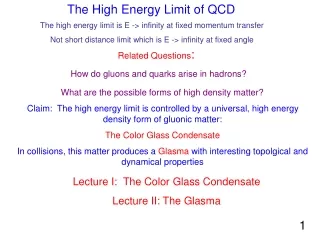
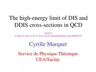
The high-energy limit of DIS and DDIS cross-sections in QCD based on Y. Hatta, E. Iancu, C.M., G. Soyez and D. Triantafyllopoulos, hep-ph/0601150 Cyrille MarquetService de Physique Théorique CEA/Saclay
Contents • Introductionkinematics and notations • The Good and Walker picture realized in pQCD- eigenstates of the QCD S-matrix at high energy: color dipoles- the virtual photon expressed in the dipole basis- inclusive and diffractive cross-sections in terms of dipole amplitudes • High-energy QCD predictions for DIS and DDIS- the geometric scaling regime- the diffusive scaling regime- consequences for the inclusive and diffractive cross-sections • Conclusionstowards the LHC
photon virtuality Q2 = - (k-k’)2 > 0 *p collision energy W2 = (k-k’+p)2 k’ some events are diffractive k diffractive mass of the final state: MX2 = (p-p’+q)2 size resolution 1/Q p p’ xpom = x/ rapidity gap: = ln(1/xpom) the diffractive cross-section: DDIS(, xpom, Q2) high-energy limit: xpom<<1 Kinematics and notations Q >> QCD Bjorken x: the *p total cross-section:DIS(x, Q2) high-energy limit: x << 1
target which remains intact the final state is then some multi-particule state : eigenstates of the interaction which can only scatter elastically elastic scattering amplitude: Description of diffractive events Good and Walker (1960) picture in the target rest frame: after the collision: hadronic particules hadronic projectile before the collision
In the high-energy limit, eigenstates are simple, provided a Fourier transform of the transverse momenta: color singlet combinations of quarks and gluons. For instance: colorless quark-antiquark pair: x, y, z: transverse coordinates colorless quark-antiquark-gluon triplet: In the large-Nc limit, further simplification: the eigenstates are only made of dipoles other quantum numbers aren’t explicitely written , the eigenvalues depend only on the transverse coordinates Eigenstates of the QCD S-matrix In general, we don’t know , and Degrees of freedom of perturbative QCD: quarks and gluons Eigenstates? The interaction should conserve their spin, polarisation, color, momentum …
x k wavefunction computed from QED at lowest order in em For instance, the component: -k y k: quark transverse momentum with transverse coordinates: x: quark transverse coordinate y: antiquark transverse coordinate The virtual photon inthe dipole basis (I) For an arbitrary hadronic projectile, we don’t know For the virtual photon in DIS and DDIS, we do know them: the wavefunction of the virtual photon is computable from perturbation theory. To describe higher-mass final states, we need to include states with more dipoles
x z y from QCD at order gS Large-Nc limit: we include an arbitrary number of gluons in the photon wave function x z1 … In principle, all are computable from perturbation theory N-1 gluons emitted at transverse coordinates N dipoles zN-1 y The virtual photon inthe dipole basis (II) With the component:
Y0 Y arbitrary Two consequences: - One can use the simplest expression (obtained for Y0 = 0) with - One can derive an hierarchy of evolution equations for the dipole amplitudes see talk by G. Soyez yesterday and previous talk by E. Iancu Formula for DIS(x, Q2) Via the optical theorem: DIS(x, Q2) = 2 Im[Ael(x, Q2)]: average over the target wave function Y = ln(1/x): the total rapidity Y0 specifies the frame in which the cross-section has been calculated, therefore DISis independent of Y0
now we need all the = ln(1/xpom) the are easily computable with a Monte Carlo Salam (1995) but we need to solve the hierarchy (or the equivalent Langevin equation) see yesterday’s talk by G. Soyez in the structure function session Formula for DDIS(, xpom, Q2) For the diffractive cross-section one obtains: new factorization formula ln(1/ )
Y - The diffractive cross-section for smaller 1, but not too small (with only the and components): • When making the assumption , we also • recover the evolution equation for Kovchegov and Levin (2000) Recovering known results - The diffractive cross-section for close to 1: same for total and diffractive cross-section (and also exclusif processes, jet production…)
High-energy QCD predictions forthe DIS and DDIS cross-sections
The dipole scattering amplitudes As explained in the previous talk by E. Iancu: • The dipole amplitudes , , … should be obtained from the recently • derived Pomeron-loop equation • This is a Langevin equation, for an event-by-event dipole amplitude , • the physical amplitudes , … are them obtained from after proper • averaging • Although one cannot solve this equation yet, some properties of the solutions have • been obtained, exploiting the similarities between the Pomeron-loop equation and • the s-FKPP equation well-known in statistical physics Mueller and Shoshi (2004); Iancu and Triantafyllopoulos (2005); Mueller, Shoshi and Wong (2005) Iancu, Mueller and Munier (2005) C.M., R. Peschanski and G. Soyez, hep-ph/0512186
at higher energies, a new scaling takes over : diffusive scaling due to the fluctuations which have been amplified as the energy increased In the diffusive scaling regime, saturation is the relevant physics up to momenta much higher than the saturation scale The different high-energy regimes in an intermediate energy regime, it predicts geometric scaling: HERA it seems that HERA is probing the geometric scaling regime
saturation models with the features of this regime fit well F2 data Golec-Biernat and Wüsthoff (1999) Bartels, Golec-Biernat and Kowalski (2002) Iancu, Itakura and Munier (2003) and they give predictions which describe accurately a number of observables at HERA (F2D, FL, DVCS, vector mesons) and RHIC (nuclear modification factor in d-Au) see yesterday’s talk by H. Kowalski The geometric scaling regime Stasto, Golec-Biernat and Kwiecinski (2001) this is seen in the data with 0.3
Y2 >Y1 Y1 The dipole amplitude is a function of one variable: We even know the functional form for : the smallest size controls the correlators The diffusive scaling regime Blue curves: different realizations of Red curve: the physical amplitude : average speed D : diffusion coefficient
total diffusive scaling geometric scaling regime: diff total geometric scaling diff DIS dominated by relatively hard sizes DDIS dominated by semi-hard sizes integrand diffusive scaling regime: both DIS and DIS are dominated by hard sizes yet saturation is the relevant physics Consequences on the observables dipole size dipole size r
And for the diffractive cross-section (integrated over at fixed x) Physical consequences: up to momentaQ²much bigger than the saturation scale • the cross-sections are dominated by small dipole sizes • there is no Pomeron (power-like) increase • the diffractive cross-section is dominated by the scattering of the quark-antiquark component Some analytic estimates Analytical estimates for DIS(x, Q2) in the diffusive scaling regime: valid for with and
Conclusions and Outlook • QCD in the high-energy limit provides a realization of the Good and Walker picture, and allows to make accurate QCD predictions for diffractive observables • From the recently-derived Pomeron-loop equation, a new picture emerges for DIS. • In an intermediate energy regime: geometric scaling- inclusive and diffractive experimental data indicate that HERA probes this regime • At higher energies: diffusive scaling - up to values of Q² much higher than the saturation scale , saturation is the relevant physics- cross-sections are dominated by rare events, in which the photon hits a black spot, that he sees dense (at saturation) at the scale Q²- the features expected when are extended up to much higherQ² • Towards the LHC- the energy there may be high enough to see the diffusive scaling regime- we want to say more before LHC starts: determination of and D ? work in progress