Download
1 / 21
210 likes | 370 Views
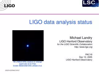
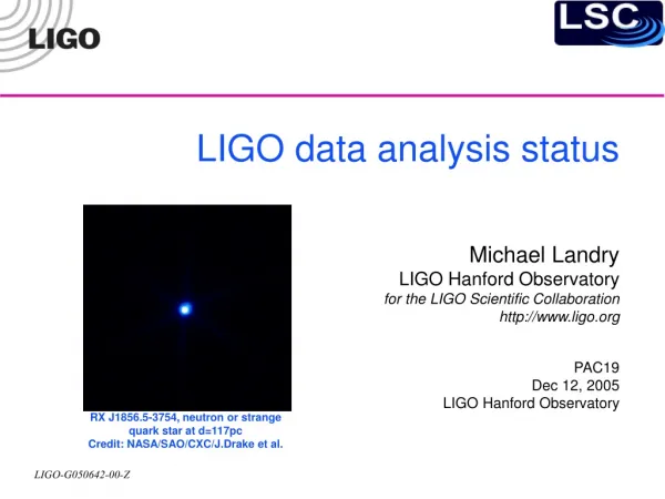
The search for continuous gravitational waves: analyses from LIGO’s second science run Michael Landry LIGO Hanford Observatory on behalf of the LIGO Scientific Collaboration http://www.ligo.org April APS Meeting (APR04) May 1-4, 2004 Denver, CO. Photo credit: NASA/CXC/SAO. Talk overview .

E N D
The search for continuous gravitational waves: analyses from LIGO’s second science runMichael LandryLIGO Hanford Observatoryon behalf of the LIGO Scientific Collaborationhttp://www.ligo.orgApril APS Meeting (APR04)May 1-4, 2004Denver, CO Photo credit: NASA/CXC/SAO
Talk overview • Introduction to continuous wave (CW) sources • CW search group analysis efforts • Review of first science run (S1) results, and a look at expectations of the S2 run • Time-domain analysis method • Injection of fake pulsars • Results
CW sources • Nearly-monochromatic continuous sources of gravitational waves include neutron stars with: • spin precession at ~frot • excited oscillatory modes such as the r-mode at 4/3 * frot • non-axisymmetric distortion of crystalline structure, at 2frot • Limit our search to gravitational waves from a triaxial neutron star emitted at twice its rotational frequency (for the analysis presented here, only) • Signal would be frequency modulated by relative motion of detector and source, plus amplitude modulated by the motion of the antenna pattern of the detector
Source model • F+ and Fx : strain antenna patterns of the detector to plus and cross polarization, bounded between -1 and 1 • Here, signal parameters are: • h0 – amplitude of the gravitational wave signal • y – polarization angle of signal • i – inclination angle of source with respect to line of sight • f0 – initial phase of pulsar; F(t=0), and F(t)= f(t) + f0 The expected signal has the form: PRD 58 063001 (1998) Heterodyne, i.e. multiply by: so that the expected demodulated signal is then: Here, a = a(h0, y, i, f0), a vector of the signal parameters.
CW search group efforts • S2 Coherent searches • Time-domain method (optimal for parameter estimation) • Target known pulsars with frequencies (2frot) in detector band • Frequency-domain F-statistic* method (optimal for blind detection) • All-sky, broadband search, subset of S2 dataset • Targeted searches (e.g. galactic core) • LMXB (e.g. ScoX-1) search • S2 Incoherent searches • Hough transform method • Powerflux method • Stackslide method • Future: Implement hierarchical analysis that layers coherent and incoherent methods • Einstein@home initiative for 2005 World Year of Physics *not the F-statistic associated with statistical literature (ratio of two variances), nor the F-test of the null hypothesis (See PRD 58 063001 (1998))
First science run: S1 • S1 run: 17 days (Aug 23-Sep 9 02) • Coincident run of four detectors, LIGO (L1, H1, H2), and GEO600 • Two independent analysis methods (frequency-domain and time-domain) employed • Set 95% upper limit values on continuous gravitational waves from single pulsar PSR J1939+2134, using LIGO and GEO IFO’s: best limit from Livingston IFO: • Accepted for publication in Phys Rev D 69, 082004 (2004), preprint available, gr-qc/0308050
S2 expectations • Coloured spectra: average amplitude detectable in time T (1% false alarm, 10% false dismissal rates): • Solid black lines: LIGO and GEO science requirement, for T=1 year • Circles: upper limits on gravitational waves from known EM pulsars, obtained from measured spindown (if spindown is entirely attributable to GW emission) • Only known, isolated targets shown here GEO LIGO
Time-domain analysis method • Perform time-domain complex heterodyne (demodulation) of the interferometer gravitational wave channel • Low-pass filter these data • The data is downsampled via averaging, yielding one value (“Bk”) of the complex time series, every 60 seconds • Determine the posterior probability distribution (pdf) of the parameters, given these data (Bk) and the model (yk) • Marginalize over nuisance parameters (cosi, j0, y) to leave the posterior distribution for the probability of h0 given the data, Bk • We define the 95% upper limit by a value h95 satisfying: 1 PDF 0 Such an upper limit can be defined even when signal is present h95 strain
noise Bk’s are processed data Bayesian analysis A Bayesian approach is used to determine the posterior distribution of the probability of the unknown parameters via the Likelihood (assuming gaussian noise within our narrow band): The posterior pdf is likelihood prior posterior model
Marginalizing over noise As we estimate the noise level from the Bk no independent information is lost by treating it as another nuisance parameter over which to marginalize, i.e. We assign Jeffreys prior to sigma, so that giving a (marginalized) likelihood of which can be evaluated analytically for gaussian noise.
Analysis summary Heterodyne, lowpass, average, calibrate: Bk Raw Data Compute likelihoods Model: yk uniform priors on h0(>0), cosi, j0, y Compute pdf for h0 Compute upper limits
S2 hardware signal injections • Performed end-to-end validation of analysis pipeline by injecting simultaneous fake continuous-wave signals into interferometers • Two simulated pulsars were injected in the LIGO interferometers for a period of ~ 12 hours during S2 • Fake signal is sum of two pulsars, P1 and P2 • All the parameters of the injected signals were successfully inferred from the data
Preliminary results for P1 Parameters of P1: P1: Constant Intrinsic Frequency Sky position: 0.3766960246 latitude (radians) 5.1471621319 longitude (radians) Signal parameters are defined at SSB GPS time 733967667.026112310 which corresponds to a wavefront passing: LHO at GPS time 733967713.000000000 LLO at GPS time 733967713.007730720 In the SSB the signal is defined by f = 1279.123456789012 Hz fdot = 0 phi = 0 psi = 0 iota = p/2 h0 = 2.0 x 10⁻²¹
Preliminary results for P2 Parameters for P2: P2: Spinning Down Sky position: 1.23456789012345 latitude (radians) 2.345678901234567890 longitude (radians) Signal parameters are defined at SSB GPS time: SSB 733967751.522490380, which corresponds to a wavefront passing: LHO at GPS time 733967713.000000000 LLO at GPS time 733967713.001640320 In the SSB at that moment the signal is defined by f=1288.901234567890123 fdot = -10-8 [phase=2 pi (f dt+1/2 fdot dt^2+...)] phi = 0 psi = 0 iota = p/2 h0 = 2.0 x 10⁻²¹
Pulsar timing • Analyzed 28 known isolated pulsars with 2frot > 50 Hz. • Timing information has been provided using radio observations collected over S2/S3 for 18 of the pulsars (Michael Kramer, Jodrell Bank). • Timing information from the Australia Telescope National Facility (ATNF) catalogue used for 10 pulsars • An additional 10 isolated pulsars are known with 2frot > 50 Hz but the uncertainty in their spin parameters is such that a search over frequency is warranted • Crab pulsar heterodyned to take timing noise into account
L1 H1 H2 joint Preliminaryresults for PSR B0021-72L • Posterior probability density for PSR J1910-5959D • Flat prior for h0 (h0>0), Jeffreys prior for s, i.e. p(s) 1/s
L1 H1 H2 joint Preliminaryresults for the Crab pulsar • Posterior probability density for PSR B0531+21 • Crab pulsar heterodyned to take timing noise into account • Flat prior for h0 (h0>0), Jeffreys prior for s, i.e. p(s) 1/s
Preliminaryupper limits for 28 known pulsars Blue: timing checked by Jodrell Bank Purple: ATNF catalogue
Equatorial Ellipticity • Results on h0 can be interpreted as upper limit on equatorial ellipticity • Ellipticity scales with the difference in radii along x and y axes • Distance r to pulsar is known, Izz is assumed to be typical, 1045 g cm2
Preliminaryellipticitylimits for 28 known pulsars Blue: timing checked by Jodrell Bank Purple: ATNF catalogue
Summary and future outlook • S2 analyses • Time-domain analysis of 28 known pulsars complete • Broadband frequency-domain all-sky search underway • ScoX-1 LMXB frequency-domain search near completion • Incoherent searches reaching maturity, preliminary S2 results produced • S3 run • Time-domain analysis on more pulsars, including binaries • Improved sensitivity LIGO/GEO run • Oct 31 03 – Jan 9 04 • Approaching spindown limit for Crab pulsar