Introduction to Robotics cpsc - 460
Introduction to Robotics cpsc - 460. Lecture 5B – Control. Control Problem. Determine the time history of joint inputs required to cause the end-effector to execute a command motion. The joint inputs may be joint forces or torques. Control Problem.

Introduction to Robotics cpsc - 460
E N D
Presentation Transcript
Introduction to Roboticscpsc - 460 Lecture 5B – Control
Control Problem • Determine the time history of joint inputs required to cause the end-effector to execute a command motion. • The joint inputs may be joint forces or torques.
Control Problem • Given: A vector of desired position, velocity and acceleration. • Required: A vector of joint actuator signals using the control law.
Robot Motion Control (I) • Joint level PID control • each joint is a servo-mechanism • adopted widely in industrial robot • neglect dynamic behavior of whole arm • degraded control performance especially in high speed • performance depends on configuration
Robot Motion Control (II) – Computed Torque • The dynamic model of the robot has the form: • is the torque about zk,if joint k is revolute joint and is a force if joint k is prismatic joint Where: M(Θ) is n x n inertia matrix, is n x 1 vector of centrifugal terms G(Θ) is a n x 1 vector of gravity terms
PD control • The control law takes the form Where:
Model based control • The control law takes the form: • Kp and KD are diagonal matrices.
Evaluating the response overshoot steady-state error ss error -- difference from the system’s desired value settling time overshoot -- % of final value exceeded at first oscillation rise time -- time to span from 10% to 90% of the final value settling time -- time to reach within 2% of the final value rise time
(x , y) 2 l2 l1 1 Project • The equations of motion:
ProjectSimulation and Dynamic Control of a 2 DOF Planar Robot • Problem statement: • The task is to take the end point of the RR robot from (0.5, 0.0, 0.0) to (0.5, 0.3, 0.0) in the in a period of 5 seconds. • Assume the robot is at rest at the starting point and should come to come to a complete stop at the final point. • The other required system parameters are: L1 = L2 = 0.4m, m1 = 10kg, m2 = 7kg, g = 9.82m/s2.
Project • Planning • Perform inverse position kinematic analysis of the serial chain at initial and final positions to obtain (1i, 2i) and (1f, 2f). • Then, obtain fifth order polynomial functions for 1 and 2 as functions of time such that the velocity and acceleration of the joints is zero at the beginning and at the end. These fifth order polynomials can be differentiated twice to get the desired velocity and acceleration time histories for the joints.
Project • Use a PD control law where Kp and Kv are 2x2 diagonal matrices, and s is the current(sensed) value of the joint angle as obtained from the simulation. Tune the control gains to obtain good performance
(x , y) 2 l2 l1 1 2DOF Robot • The forward kinematic equations: • The inverse kinematic equations: • The Jacobian matrix