Download
1 / 1
10 likes | 97 Views
This article discusses the replacement of trial-and-error image matching with direct object parameter retrieval, utilizing linearization and regularization techniques in dynamical scattering theory. The challenges of stabilization, parameter inclusion, and extension to mixed potential approximations are addressed. Examples include reconstruction of tilted and twisted grains in materials like Au and GeCdTe. The article proposes perturbation solutions, likelihood measures, and regularization methods for accurate parameter determination and potential inversion. It aims to recover potential variations in three dimensions and improve modeling accuracy.

E N D
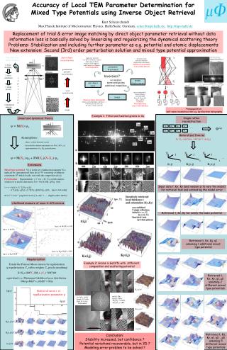
A000 A1-11 A1-1-1 1. object modeling Kx(i,j)/a* 2. wave simulation A-111 A-11-1 A-220 object wave amplitude r e p e t i t i o n FT set q1: Ge set q2: CdTe dVo/Vo = 0.02% dV’o/V’o = 0.8% Ge-CdTe, 300kV Sample: D. Smith Holo: H. Lichte, M.Lehmann ? 3. image process wave reconstruction Ky(i,j)/a* ? P000 P1-11 P1-1-1 4. likelihood measure image 10nm object wave phase t(i,j)/Å P-111 P-11-1 P-220 trial-and-error image analysis direct object reconstruction parameter & potential reconstruction y = M(X) y0 Assumptions: - object: weakly distorted crystal - described by unknown parameter set X={t, K,Vg, u} - approximations of t0, K0 a priori known y = M(X0) y0 + JM(X0)(X-X0) y0 ... A0 Ag1 Ag2 Ag3 Fexp ... P0 Pg1 Pg2 Pg3 X= X0+(JMTJM)-1JMT.[Fexp- F(X0)] X X X j j j ... i i i t(i,j) Kx(i,j) Ky(i,j) Kurt Scheerschmidt Max Planck Institute of Microstructure Physics, Halle/Saale, Germany, schee@mpi-halle.de, http://mpi-halle.de Replacement of trial & error image matching by direct object parameter retrieval without data information loss is basically solved by linearizing and regularizing the dynamical scattering theory Problems: Stabilization and including further parameter as e.g. potential and atomic displacements New extension: Second (3rd) order perturbation solution and mixed type potential approximation multi-slice inversion (van Dyck, Griblyuk, Lentzen, Allen, Spargo, Koch) Pade-inversion (Spence) non-Convex sets (Spence) local linearization Accuracy of Local TEM Parameter Determination for Mixed Type Potentials using Inverse Object Retrieval deviations from reference structures: displacement field (Head) algebraic discretization no succesful test yet parameter & potential Inversion? atomic displacements exit object wave direct interpretation : Fourier filtering QUANTITEM Fuzzy & Neuro-Net Srain analysis however: Information loss due to data reduction image reference beam (holography) defocus series (Kirkland, van Dyck …) Gerchberg-Saxton (Jansson) tilt-series, voltage variation Presupposition: exit wave reconstruction e.g. by electron holography Example 1: Tilted and twisted grains in Au Single reflex reconstruction Linearized dynamical theory Generalized Inverse Extensions Mixed type potential: V(i,j) in the set of unknown parameter X is replaced by a parametrized form qk(i,j)*Vk consisting of different constituents Vk which locally vary with the composition qk(i,j) • Perturbation: Eigensolution g, C for t, K, V, q yields analytic solution of y and its derivatives for t +dt, K+dK, q+dq, with • = g + tr(D) + D-1{1/(gi-gj)}D - D-1{Dii/(gi-gj)2}D +D-1{1/(gi-gj)}D{1/(gi-gk)}D (up to 3rd order) • M = C-1(1+D)-1 {exp(2pil(t+Dt)} (1+D)C +… (higher order simile) no iteration same ambiguities additional instabilities Input data t, Kx, Ky (and random qi to vary the model) for retrieval test and estimating the model error Likelihood measure of wave F differences Retrieved t, Kx, Ky for solely the basic potential log(e) of F(dX) vs |dX| log(e) of F(dX) Retrieved t, Kx, Ky, q1 assuming 1 additional mixed type potential log(e) of F0+dXdF vs |dX| log(e) of F0+dXdF Regularization Example 2: Grains in GeCdTe with different composition and scattering potential Extend the Penrose-Moore inverse by regularization (r regularization, C1 reflex weights, C2 pixels smoothing) X=X0+(JMTC1JM + rC2)-1JMTDF equivalent to a Maximum-Likelihood error distribution: ||Fexp-Fth||2 + r||DX||2 = Min Retrieved t, Kx, Ky, q1, q2 assuming 2 different mixed type potentials 3 4 5 Retrieval error e vs regularization parameter r lg(e) -lg(r) 3 4 Kx(i,j)/a* 5 Ky(i,j)/a* Retrieved t, Kx, Ky, q1, q2,…,q5 assuming 5 different mixed type potentials Conclusion: Stability increased, but confidence ? Potential variations recoverable, but in 3D ? Modeling error problem to be solved ? t(i,j)/Å