Download
1 / 13
130 likes | 150 Views
This article explains the concepts of barotropic and baroclinic flows in the ocean, their characteristics, and the relationships between isobaric and isopycnal surfaces and currents. It also discusses the accuracy of measurements and provides examples of sea surface height and thermocline depth anomalies.

E N D
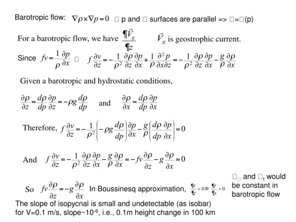
Barotropic flow: p and surfaces are parallel => =(p) For a barotropic flow, we have is geostrophic current. Since Given a barotropic and hydrostatic conditions, and Therefore, And and twould be constant in barotropic flow So In Boussinesq approximation, The slope of isopycnal is small and undetectable (as isobar) for V=0.1 m/s, slope~10-6, i.e., 0.1m height change in 100 km
Relations between isobaric and isopycnal surfaces and currents Baroclinic Flow: and There is no simple relation between the isobars and isopycnals. slope of isobar is proportional to velocity slope of isopycnal is proportional to vertical current shear. With a barotropic of mass the water may be stationary but with a baroclinic field, having horizontal density gradients, such situation is not possible In the ocean, the barotropic case is most common in deep water while the baroclinic case is most common in the upper 1000 meters where most of the faster currents occur.
1 and 1/2 layer flow Simplest case of baroclinic flow: Two layer flow of density 1 and 2. The sea surface height is =(x,y) (In steady state, =0). The depth of the upper layer is at z=d(x,y)<0. The lower layer is at rest. For z > d, For z ≤ d, If we assume The slope of the interface between the two layers (isopycnal)= times the slope of the surface (isobar). The isopycnal slope is opposite in sign to the isobaric slope.
Why is the slope of dynamical height more easily determined than the slope of isobar? slope of isopycnal surface Density difference in the ocean is small and so isopycnal slope is magnified from isobaric slope by a factor of ρ/Δρ Accuracy of measurement: Depth ±1 in 103 Density ±5 in 106
σt A B diff 26.8 50m --- >50m 27.0 130m 280m -150m 27.7 570m 750m -180m Isopycnals are nearly flat at 100m Isobars ascend about 0.13m between A and B for upper 150m Below 100m, isopycnals and isobars slope in opposite directions with 1000 times in size.
Relation between fluctuations of SSH () and thermocline depth (h) 20oC isotherm anomalies (m) COLA ODA December,1997-February, 1998 SSH anomalies (cm) TOPEX/Poseidon
Example: sea surface height and thermocline depth“Warm water on the right”
Comments on the geostrophic equation • If the ocean is in “real” geostrophy, there is no water parcel acceleration. No other forces acting on the parcel. Current should be steady • Present calculation yields only relative currents and the selection of an appropriate level of no motion always presents a problem • One is faced with a problem when the selected level of no motion reaches the ocean bottom as the stations get close to shore • It only yields mean values between stations which are usually tens of kilometers apart • Friction is ignored • Geostrophy breaks down near the equator (within 0.5olatitude, or ±50km) • The calculated geostrophic currents will include any long-period transient current