Download
1 / 36
360 likes | 467 Views
Climate Change: Addressing Uncertainty, Inertia, and Equity. The Greenhouse Effect E. Boeker, Environmental Physics # updated for 2005 ann.average CO2 conc. CDIAC. Gas conc. ppm GWP factor G. Warming (ºK)

E N D
Climate Change: Addressing Uncertainty, Inertia, and Equity Arnulf Grubler
The Greenhouse EffectE. Boeker, Environmental Physics#updated for 2005 ann.average CO2 conc. CDIAC Gas conc. ppm GWP factor G. Warming (ºK) H2O 5000 0.2 20.6 CO2 380# 1 7.2O3 0.03 3900 2.4 N2O 0.3 310 0.8 CH4 1.7 21 0.8 HFC-134 ~ 0.03 1000 0.6 Total 32.4 Arnulf Grubler
Source: IPCC AR4 WG1 2007 Arnulf Grubler
Temperature Change (over 1901-1950 mean): Observations and Modeled by Including all Positive and Negative Forcings. Source: IPCC AR4 WG1 2007 Arnulf Grubler
EU Regional Climate Variability:Observations (b)modeled for present (c)and future (d)conditions.Note 2003 heat wave (a) being far outside both observational and model range.IPCC uncertainty terminology (adopted from Schneider and Moss) :<1% probability =“exceptionally unlikely” (but 2003 happened)
Height of Pasterze glacier in 1960 Current CC Impacts: 80 meters thinning of Pasterze glacier, Austria But…uncovering 5000 yrold vegetation
Global Carbon & Warming Budgets Arnulf Grubler
Climate Change: Major Uncertainties • Demographic (growth & composition) • Economic (growth, structure, disparities) • Social(values, lifestyles, policies) • Technologic (rates & direction of change) • Environmental (limits, adaptability) • Valuation (discounting, non-market damages and benefits) • Addressing uncertainties: Scenarios Research Social choice Arnulf Grubler
A Taxonomy of SRES Scenarios(“baselines”, no climate policies) Arnulf Grubler
Emissions vs. Energy Use & Technologyin IPCC SRES Scenarios Uncertainty 2: Resource availability, technology Uncertainty 1: Population and GDP growth, prices, policies
Example Climate Change:Projected Global Mean Temperature Change and Sources of Uncertainty IPCC WG1 TAR: “By 2100, the range in the surface temperature response across the group of climate models run with a given scenario is comparable to the range obtained from a single model run with the different SRES scenarios”
Example Climate Change:Projected Global Mean Temperature Change and Sources of Uncertainty Baseline Uncertainty: 50 % climate (sensitivity) modeling25% emissions (POP+GDP influence)25% emissions (TECH influence) Uncertainty on extent and success of climate policies Minimum committed warming1.5 °C (certainty)
MAJOR CLIMATE CHANGE UNCERTAINTIESSocioeconomic (Future Cumulative Emissions SRES Scenarios)Carbon Cycle (Resulting CO2 Concentration) andClimate Sensitivity (ºC for 2CO2) ° C global mean temperature change 1 2 3 4 5 6 0 2.5 7 ppm CO2 300 600 1000 6 4 2 0 2000 3000 <100 1000 SRES scenarios cumulative emissions 1990 - 2100, GtC low high Vulnerability:
Uncertainties (F=carbon cycle; Δt2x=climate sensitivity)in Stabilizing Climate Change at +2.5 ºC by 2100 20 10,000 (b) (a) (2.6, 1.5) 1,000 15 ) (2.6, 2.5) 1 - 100 10 shadow price ($ per ton C) Carbon emissions (GtC yr (0.6, 4.5) 10 (1.1, 2.5) 550 ppmv ( F = 1.1) 550 ppmv ( F = 1.1) 550 ppmv ( F = 0.6) 5 2 550 ppmv ( F = 0.6) 550 ppmv ( F = 2.6) CO 1 (0.6, 2.5) 550 ppmv ( F = 2.6) D F = 0.6 T = 4.5 2x D F = 0.6 T = 4.5 D F = 2.6 T = 1.5 2x 2x D F = 2.6 T = 1.5 (not shown as zero) 2x 0.1 0 1990 2000 2010 2020 2030 2040 2050 2060 2070 2080 2090 2100 1990 2000 2010 2020 2030 2040 2050 2060 2070 2080 2090 2100 Year Year Emissions Shadow Prices
North -- South • Responsibility: Mostly in Annex-I • Vulnerability: Mostly in “South” • Adaptation capacity: Mostly in Annex-I • Future emission growth: Mostly in “South” • Near-term mitigation potential: highest in Annex-I • Near-term mitigation costs: lowest in “South” Arnulf Grubler
1990 Per Capita CO2 by Source vs. Population Arnulf Grubler
The Greenhouse “Barometer” Arnulf Grubler
Agricultural Impacts for Alternative Climate Change Scenarios. Source: IIASA LUCC, 2000. Arnulf Grubler
Environmental Change: Development vs. Climate • More ecosystems will be destroyed by economic development than by the climate change this development induces • Far more human lives are threatened by a lack of development than by any climate change resulting from a closure of the development gap • Baselines: “business-as-usual” + climate control vs sustainability paradigm Arnulf Grubler
Vulnerability to Economic Development vs. Seal Level Rise. Source: IPCC AR4 WG2, 2007 Arnulf Grubler
Reducing CC Vulnerabilities • Economic & Social Developmentun-targeted and asymmetricalpoverty vulnerability: -affluence vulnerability: + • Adaptation targeted to CC • Emissions reduction (mitigation)lowering CC but not eliminating it Arnulf Grubler
Vulnerability to CC by 2050 (IPCC AR4 WG2 2007) A2 current adaptive capacity Improved adaptive capacity Mitigation only (550 stab) Mitigation + improved adaptation Arnulf Grubler
Mitigation Options • Demographic change • Economic development • Social behavior • Efficiency Improvements • Low carbon intensity • Zero carbon (solar, nuclear) • Carbon removal • Non CO2 gases (agriculture&industry) • End deforestation • Sink enhancements • “geo-engineering” Arnulf Grubler
Emissions & Reduction MeasuresMultiple sectors and stabilization levels Source: Riahi et al., TFSC 2007 Arnulf Grubler
Costs of Different Baselines and Stabilization ScenariosSource: IIASA, 2000. Deployment rate of efficiency and low-emission technologies Σ: The lower baseline emissions (efficiency, clean supply)the easier to achieve (currently unknown) climate targets
Stabilization Costs(% GDP loss, top,; and carbon price, $/tCO2, bottom) by 2100 as a Function of Baseline, Model, and Stabilization Level DifferencesIPCC AR4 WG3 2007
Technology as Source and Remedy of Climate Change:IPCC Baselines and 550 ppmv Stabilization Scenarios (in GtC), Source: IIASA, 2002. BASELINE WITHFROZEN EFFICIENCY AND TECHNOLOGY Σ: With “frozen” efficiency and technology improvementsemissions grow “through the roof”. Even with continued improvements,additional emission reduction is needed for climate stabilization
Baseline Emissions vs. Reductions in Illustrative 550 ppm Stabilization Scenarios (Source: Riahi, 2002) Σ: The higher the baseline emissions, the more reliance on “silver bullet” backstop technologies like CCS
Emission Reduction Measures Riahi et al. TFSC 2007 Improvements incorporated in baselines Emissions reductions due to climate policies Σ: Technological change in Baseline best hedging against target uncertainty
Emission Reduction Measures Riahi et al TFSC 2007 (0.9 incl. baseline) RF = Robustness factor of options across scenario uncertainty is highest for:F-gases and N2O reduction, energy conservation & efficiency, and biomass+CCS “wildcard” (if feasible)
Mitigation Technology Portfolio Analysis • Paramount importance of Baseline • Costs matter • Diffusion time constants matter • Differences in where technology is developed and where it is deployed • Technological interdependence and systemic aspects important in “transition” analysis • Non-energy, non-CO2 can help, but cannot solve problem Σ:Popular “wedge” analysis fails on all above accounts!
Energy Carbon and Climate: How far to go? • Energy: 20 (5% exergy efficiency) • Carbon: Zero (H2-economy) • Damages: committed warming (>1.5 C?) • Non-linear (catastrophic) change: ??? • “Collateral damages”-- Geoengineering, e.g. aerosol cooling (white sky)-- sequestration (leakage, marine ecology)-- biomass (soil carbon, biodiversity, agriculture)-- solar (albedo changes) Arnulf Grubler
Policy Conundrums • Equitable quantitative targets at odds with economics or infeasible • Cost optimal emission reduction: Start with inefficiencies in DCs but requires new instruments (CDM+) • Separation of equity and efficiency (e.g. via tradable permit allocation) might be politically infeasible (unprecedented N-S resource transfers) • Uncertainties cannot be ignored (soil C, avoided deforestation) • Mitigation technology innovation “recharge” chain broken (declining R&D) Arnulf Grubler
Allocating Emissions Reductions or Access to Global Commons Arnulf Grubler