Download
1 / 52
550 likes | 893 Views
Very Long Baseline Interferometry. Ylva Pihlström (UNM) Craig Walker (NRAO). Outline. What is VLBI? What is VLBI good for? How is VLBI different from connected element interferometry? What issues do we need to consider in VLBI observations?. What is VLBI?.

E N D
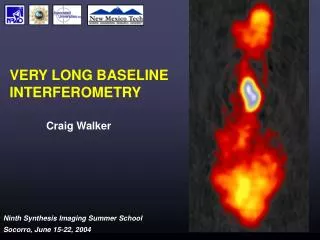
Very Long Baseline Interferometry Ylva Pihlström (UNM) Craig Walker (NRAO)
Outline • What is VLBI? • What is VLBI good for? • How is VLBI different from connected element interferometry? • What issues do we need to consider in VLBI observations?
What is VLBI? • VLBI is interferometry with disconnected elements • No fundamental difference from connected element interferometry • The basic idea is to bring coherent signals together for correlation, and to get fringes from each interferometer Connected elements: done via cables
VLBI versus connected elements • In VLBI there are no IFs or LOs connecting the antennas • Instead accurate time standards and a recording system is used Mark 5 recording system
VLBI correlators • The correlation is not real-time but occurs later on • Disks/tapes shipped to the correlators • Examples are the VLBA and the JIVE correlator
What is VLBI good for? • 'Very Long Baselines' implies high angular resolution ( ~ /B) • The Very Long Baseline Array (VLBA) 0.1 - 5 mas
Global VLBI stations From GSFC (some astronomy stations missing)
The black hole in NGC4258 • Tangential disk masers at Keplerian velocities • First real measurement of nuclear black hole mass • Add time dimension (4D) => geometric distance Image courtesy: L. Greenhill
The SS433 movie • X-ray binary with precessing relativistic jet • Daily snapshot observation with the VLBA at 20 cm for 40 days (~1/4 of precession period). Mioduszewski, Walker, Rupen & Taylor
Astrometry • 12 epochs of observations on T Tauri Sb • This has driven down the distance error to 0.8 pc Image courtesy: A. Mioduszewski, L. Loinard
10 cm Baseline Length 1984-1999 Baseline transverse 10 cm Distance from Germany to Massachusetts GSFC Jan. 2000
Differences VLBI and connected interferometry • Not fundamentally different, only issues that lead to different considerations during calibration • Rapid phase variations and gradients introduced by • Separate clocks • Independent atmosphere at the antennas • Phase stabilities varies between telescopes • Model uncertainties due to inaccurate source positions, station locations, and Earth orientation, which are difficult to know to a fraction of a wavelength • Solve by fringe fitting
Differences VLBI and connected interferometry (continued) • The calibrators are not ideal since they are a little resolved and often variable • No standard flux calibrators • No point source amplitude calibrators • Solve by using Tsys and gains to calibrate amplitudes • Only sensitive to limited scales • Structure easily resolved out • Solve by including shorter baselines (MERLIN, VLA)
Differences VLBI and connected interferometry (continued) • Only sensitive to non-thermal emission processes (Tb,min-2HPBW) • 106 K brightness temperature limit • Limits the variety of science that can be done • To improve sensitivity • Use bigger telescopes (HSA) • For continuum, use a higher data rate (wider bandwidth), MkV (disk based recording) can reach 1GBps Chapter 9 in the book
VLBI data reduction path - continuum Fringe fitting: residual delay correction Correlator Examine data Apply on-line flags Flag table Delay, rate and phase calibration Tsys table, gain curves Tsys, gain and opacity corrections Pcal: instrumental delay correction Self-calib Image Interactive editing Analysis Amplitude cal improvement
The task of the correlator • Main task is to cross multiply signals from the same wavefront • Antennas at different distances => delay • Antennas move at different speed => rate • Offset estimates removed using a geometric model • Remaining phase errors normally dominated by the atmosphere • Write out data
The VLBA delay model Adapted from Sovers, Fanselow, and Jacobs, Reviews of Modern Physics, Oct 1998.
VLBI data reduction path - continuum Fringe fitting: residual delay correction Correlator Examine data Apply on-line flags Flag table Delay, rate and phase calibration Tsys table, gain curves Tsys, gain and opacity corrections Pcal: instrumental delay correction Self-calib Image A priori Interactive editing Analysis Amplitude cal improvement
Apriori editing • Flags from the on-line system will remove bad data from • Antenna not yet on source • Subreflector not in position • LO synthesizers not locked
VLBI amplitude calibration • Scij = Correlated flux density on baseline i - j • = Measured correlation coefficient • A = Correlator specific scaling factor • s= System efficiency including digitization losses • Ts = System temperature • Includes receiver, spillover, atmosphere, blockage • K = Gain in degrees K per Jansky (includes gain curve) • e- = Absorption in atmosphere plus blockage
Calibration with system temperatures Upper plot: increased Tsys due to rain and low elevation Lower plot: removal of the effect.
VLBA gain curves • Caused by gravitationally induced distortions of antenna • Function of elevation, depends on frequency 4cm 2cm 1cm 20cm 50cm 7mm
Atmospheric opacity correction • Corrections for absorption by the atmosphere • Can estimate using Ts - Tr - Tspill Example from VLBA single dish pointing data
Instrumental delays • Caused by different signals paths through the electronics in the separate bands
The pulse cal • Corrected for using the pulse cal system (continuum only) • Tones generated by injecting a pulse every microsecond Pulse cal monitoring data Pcal tones
Corrections using Pcal • Data aligned using Pcal • No Pcal at VLA, shows unaligned phases
Ionospheric delay • Delay scales with 1/2 • Ionosphere dominates errors at low frequencies • Can correct with dual band observations (S/X) or GPS based models Maximum Likely Ionospheric Contributions Delays from an S/X Geodesy Observation -20 Delay (ns) 20 Time (Days)
GPS based ionospheric models Ionosphere map from iono.jpl.nasa.gov
VLBI data reduction path - continuum Fringe fitting: residual rate & delay correction Correlator Examine data Apply on-line flags Flag table Delay, rate and phase calibration Tsys table, gain curves Tsys, gain and opacity corrections Pcal: instrumental delay correction Self-calib Image Interactive editing Analysis Amplitude cal improvement
Editing Editing • Flags from on-line system will remove most bad data • Antenna off source • Subreflector out of position • Synthesizers not locked • Final flagging done by examining data • Flag by antenna (most problems are antenna based) • Poor weather • Bad playback • RFI (may need to flag by channel) • First point in scan sometimes bad
Editing example Raw Data - No Edits Raw Data - Edited A (Jy) (deg) A (Jy) (deg) A (Jy) (deg) A (Jy) (deg)
Amplitude check source Amplitude check source • Typical calibrator visibility function after apriori calibration • One antenna low, perhaps due to poor weather • Resolved => need to image • Use information to fine tune the amplitude calibration Resolved – a model or image will be needed Poorly calibrated antenna
VLBI data reduction path - continuum Fringe fitting: residual rate & delay correction Correlator Examine data Apply on-line flags Flag table Delay, rate and phase calibration Tsys table, gain curves Tsys, gain and opacity corrections Pcal: instrumental delay correction Self-calib Image Interactive editing Analysis Amplitude cal improvement
Phase errors • Raw correlator output has phase slopes in time and frequency • Caused by imperfect delay model • Need to find delay and delay-rate errors
Fringe fitting • For astronomy: • Remove clock offsets and align baseband channels (“manual pcal”) • Fit calibrator to track most variations • Fit target source if strong • Used to allow averaging in frequency and time • Allows higher SNR self calibration (longer solution, more bandwidth) • For geodesy: • Fitted delays are the primary “observable” • Correlator model is added to get “total delay”, independent of models
Residual rate and delay • Interferometer phase t, = 2t • Slope in frequency is “delay” • Fluctuations worse at low frequency because of ionosphere • Troposphere affects all frequencies equally ("nondispersive") • Slope in time is “fringe rate” • Usually from imperfect troposphere or ionosphere model
Fringe fitting theory • Interferometer phase t, = 2t • Phase error dt, = 2dt • Linear phase model t, = 0 + (/) + (/t)t • Determining the delay and rate errors is called "fringe fitting" • Fringe fit is self calibration with first derivatives in time and frequency
Fringe fitting: how • Usually a two step process • 2D FFT to get estimated rates and delays to reference antenna • Use these for start model for least squares • Can restrict window to avoid high sigma noise points • Least squares fit to phases starting at FFT estimate • Baseline fringe fit • Fit each baseline independently • Must detect source on all baselines • Used for geodesy. • Global fringe fit (like self-cal) • One phase, rate, and delay per antenna • Best SNR because all data used • Improved by good source model • Best for imaging and phase referencing
Self calibration imaging sequence • Iterative procedure to solve for both image and gains: • Use best available image to solve for gains (start with point) • Use gains to derive improved image • Should converge quickly for simple sources • Does not preserve absolute position or flux density scale
Phase referencing • Calibration using phase calibrator outside target source field • Nodding calibrator (move antennas) • In-beam calibrator (separate correlation pass) • Multiple calibrators for most accurate results – get gradients • Similar to VLA calibration except: • Geometric and atmospheric models worse • Model errors usually dominate over fluctuations • Errors scale with total error times source-target separation in radians • Need to calibrate often (5 minute or faster cycle) • Need calibrator close to target (< 5 deg) • Used by about 30-50% of VLBA observations
Phase referencing/self cal example • No phase calibration: source not detected • Phase referencing: detected, but distorted structure (target-calibrator separation probably large) • Self-calibration on this strong source shows real structure No Phase Calibration Reference Calibration Self-calibration
VLBI data reduction path - spectral line Fringe fitting: residual rate & delay correction Correlator Examine data Apply on-line flags Flag table Delay, rate and phase calibration Tsys table, gain curves Tsys, gain and opacity corrections Doppler correction Manual pcal: instr. delay correction Bandpass calibration Interactive editing Self-calib Image Bandpass amplitude cal. Amplitude cal improvement Analysis
Manual Pcal • Cannot use the pulse cal system if you do spectral line • Manual Pcal uses a short scan on a strong calibrator, and assumes that the instrumental delays are time-independent • In AIPS, use FRING instead of PCAL
Editing spectral line data • No difference from continuum, except for that a larger number of channels allow for RFI editing
Bandpass calibration: why • Complex gain variations across the band, slow functions of time • Needed for spectral line calibration • May help continuum calibration by reducing closure errors caused by averaging over a variable bandpass Before After
Bandpass calibration: how • Best approach to observe a strong, line-free continuum source (bandpass calibrator) • Two step process: • Amplitude bandpass calibration before Doppler corrections • Complex bandpass calibration after continuum (self-)cal on bandpass cal. • After final continuum calibration (fringe-fit) of the calibrators, good cross-correlation continuum data exists • The bandpass calibrator must be calibrated so its visibility phase is known - residuals are system • Use the bandpass calibrator to correct individual channels for small residual phase variations • Basically a self-cal on a per channel basis
Additional spectral line corrections • Doppler shifts: • Without Doppler tracking, the spectra will shift during the observations due to Earth rotation. • Recalculate in AIPS: shifts flux amongst frequency channels, so you want to do the amplitude only BP calibration first • Self-cal on line: • can use a bright spectral-line peak in one channel for a one-channel self-cal to correct antenna based temporal phase and amplitude fluctuations and apply the corrections to all channels
Preparing observations • Know the flux density of your source (preferrably from interferometry observations) • For a line target, is the redshifted frequency within the available receiver bands? Different arrays have different frequency coverage. • What angular resolution is needed for your science? Will determine choice of array. • Will you be able to probe all important angular scales? Include shorter baselines? • Can you reach the required sensitivity in a decent time?